Performing grid search in tidyflow
Source:vignettes/d04_fitting-model-tuning.Rmd
d04_fitting-model-tuning.RmdThis vignette aims to exemplify how you can use resampling and tuning within a tidyflow.
A tidyflow is a bundle of steps that allow you to bundle together your data, splitting, resampling, preprocessing, modeling, and grid search. For executing a grid search, the tidymodels ecosystem contains the tune package. tune allows you to run many sub-models, each one with a different combination of tuning parameters, with the aim of choosing the best final model.
In another vignette, we discussed the concept of resampling and how it can be used to evaluate the stability of a model. For performing a grid search, resampling is a natural step because we need to try a combination of tuning values for each parameter in a model. In other words, we will run many models with different values for the models parameters and we need a way to get random samples from the data. Resampling is thus combined with a general strategy of trying out different sub-models.
Let’s define a random forest model but we want to try different values in the trees argument. We can signal that with the tune() function. This just means that the trees will be tuned.
library(tidymodels)
library(tidyflow)

rf <- rand_forest(mode = "regression", trees = tune()) %>% set_engine("randomForest")
rf
#> Random Forest Model Specification (regression)
#>
#> Main Arguments:
#>   trees = tune()
#>
#> Computational engine: randomForest
At this point, we haven’t really ‘defined’ which values will be used for trees. It could be 3 values (such as 100, 200 and 300) or it could be 500. The package tune hosts a family of functions named grid_* which provide different approaches to sampling random number from different tuning arguments. For example, let’s use grid_regular to obtain an evenly spaced set of values for trees. This is how you would do it in tidymodels:
even_values <- grid_regular(trees(), levels = 10)
even_values
#> # A tibble: 10 x 1
#>    trees
#>    <int>
#>  1     1
#>  2   223
#>  3   445
#>  4   667
#>  5   889
#>  6  1111
#>  7  1333
#>  8  1555
#>  9  1777
#> 10  2000
grid_regular already knows which ‘sensible’ range of values to try. tidyflow provides the function plug_grid that allows you to specify the type of grid search you want to perform. Let’s divide the data into training/testing, specify a cross-validation and plug in the random forest and a grid_regular:
tflow <-
  mtcars %>%
  tidyflow(seed = 57136) %>%
  plug_formula(mpg ~ .) %>%
  plug_split(initial_split) %>%
  plug_resample(vfold_cv) %>%
  plug_model(rf) %>%
  plug_grid(grid_regular)

tflow
#> ══ Tidyflow ════════════════════════════════════════════════════════════════════
#> Data: 32 rows x 11 columns
#> Split: initial_split w/ default args
#> Formula: mpg ~ .
#> Resample: vfold_cv w/ default args
#> Grid: grid_regular w/ default args
#> Model:
#> Random Forest Model Specification (regression)
#>
#> Main Arguments:
#>   trees = tune()
#>
#> Computational engine: randomForest
This grid search specification knows that trees is the only argument to be searched for. We can execute the grid search with just a single call to fit:
res <- tflow %>% fit()
#> randomForest 4.6-14
#> Type rfNews() to see new features/changes/bug fixes.
#>
#> Attaching package: 'randomForest'
#> The following object is masked from 'package:ggplot2':
#>
#>     margin
#> The following object is masked from 'package:dplyr':
#>
#>     combine
#> ! Fold08: internal: A correlation computation is required, but `estimate` is const...
res %>% pull_tflow_fit_tuning()
#> Warning: This tuning result has notes. Example notes on model fitting include:
#> internal: A correlation computation is required, but `estimate` is constant and has 0 standard deviation, resulting in a divide by 0 error. `NA` will be returned.
#> # Tuning results
#> # 10-fold cross-validation
#> # A tibble: 10 x 4
#>    splits         id     .metrics         .notes
#>    <list>         <chr>  <list>           <list>
#>  1 <split [21/3]> Fold01 <tibble [6 × 5]> <tibble [0 × 1]>
#>  2 <split [21/3]> Fold02 <tibble [6 × 5]> <tibble [0 × 1]>
#>  3 <split [21/3]> Fold03 <tibble [6 × 5]> <tibble [0 × 1]>
#>  4 <split [21/3]> Fold04 <tibble [6 × 5]> <tibble [0 × 1]>
#>  5 <split [22/2]> Fold05 <tibble [6 × 5]> <tibble [0 × 1]>
#>  6 <split [22/2]> Fold06 <tibble [6 × 5]> <tibble [0 × 1]>
#>  7 <split [22/2]> Fold07 <tibble [6 × 5]> <tibble [0 × 1]>
#>  8 <split [22/2]> Fold08 <tibble [6 × 5]> <tibble [1 × 1]>
#>  9 <split [22/2]> Fold09 <tibble [6 × 5]> <tibble [0 × 1]>
#> 10 <split [22/2]> Fold10 <tibble [6 × 5]> <tibble [0 × 1]>
The result is a resampling object with the evaluation metrics measuring the performance of different values for trees across the 10 resamples. You can look at more clearly the performance of the model using different values for trees using autoplot() on the resampling result:
res %>% pull_tflow_fit_tuning() %>% autoplot()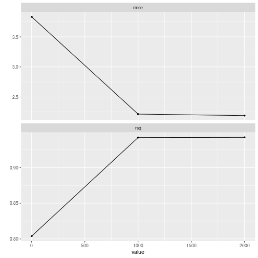
plot of chunk grid_search_tuning1
It seems the grid randomly chose three values for trees (X axis has three points on 1, 1000 and 2000) and as expected, as the number of trees increases, the rsq is higher and the rmse is lower.
This grid search strategy is really just a quick way to get some models running. However, it allows for much more flexibility. For example, we can play around with the number of values to sample from by just providing an extra argument to plug_grid:
tflow <-
  mtcars %>%
  tidyflow(seed = 57136) %>%
  plug_formula(mpg ~ .) %>%
  plug_split(initial_split) %>%
  plug_resample(vfold_cv) %>%
  plug_model(rf) %>%
  plug_grid(grid_regular, levels = 10)

tflow %>%
  fit() %>%
  pull_tflow_fit_tuning() %>%
  autoplot()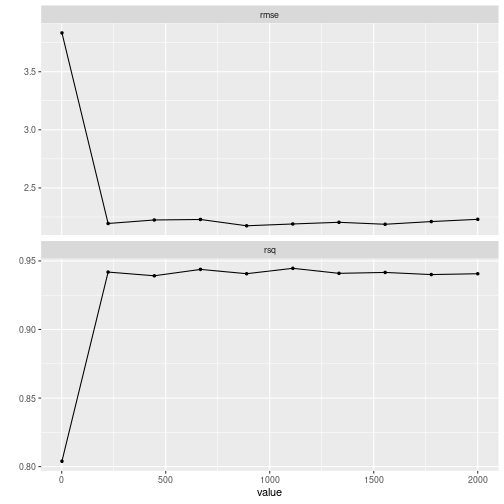
plot of chunk grid_search_tuning2
The random grid contains now 10 values. What if we wanted to limit the range of the values used in the resampling?
tflow <-
  mtcars %>%
  tidyflow(seed = 57136) %>%
  plug_formula(mpg ~ .) %>%
  plug_split(initial_split) %>%
  plug_resample(vfold_cv) %>%
  plug_model(rf) %>%
  plug_grid(grid_regular, trees = trees(range = c(1, 20)), levels = 10)

tflow %>%
  fit() %>%
  pull_tflow_fit_tuning() %>%
  autoplot()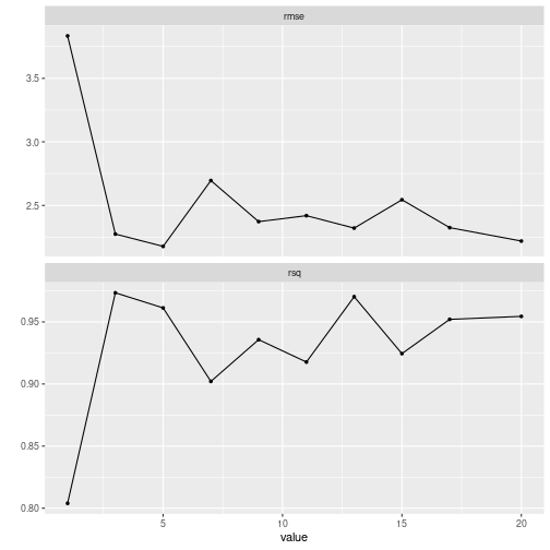
plot of chunk grid_search_tuning3
This approach works just as well with any of the grid_* functions. However, what if we simply wanted to provide the values to try? That is, we don’t want any type of ‘random sampling’. plug_grid allows the user to specify the function expand.grid and just provide the values to be used in the grid search. For example:
tflow <-
  mtcars %>%
  tidyflow(seed = 57136) %>%
  plug_formula(mpg ~ .) %>%
  plug_split(initial_split) %>%
  plug_resample(vfold_cv) %>%
  plug_model(rf) %>%
  plug_grid(expand.grid, trees = c(1, 5, 10))

tflow %>%
  fit() %>%
  pull_tflow_fit_tuning() %>%
  autoplot()
#> Warning: Duplicate rows in grid of tuning combinations found and removed.
#> ! Fold08: internal: A correlation computation is required, but `estimate` is const...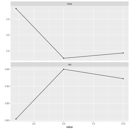
plot of chunk grid_search_tuning4
This flexibility works just as well with any number of tuning parameters for the model. You can specify as many as parameters as you want, and even manually customize some of the parameters while the grid_* functions takes care of randomly sampling the others. For example, let’s say we wanted to run a random forest while tuning the parameters trees, min_n and mtry. Suppose that on top of that we wanted to manually limit the range of trees to be between 5 and 20, the min_n to be 20 (fixed) and allow the grid sampling to sample mtry randomly from ‘sensible’ values. We do that just as we’ve been manually updating the parameters values in plug_grid:
rf <-
  rand_forest(mode = "regression",
              trees = tune(),
              min_n = 20,
              mtry = tune()) %>%
  set_engine("randomForest")

tflow <-
  mtcars %>%
  tidyflow(seed = 57136) %>%
  plug_formula(mpg ~ .) %>%
  plug_split(initial_split) %>%
  plug_resample(vfold_cv) %>%
  plug_model(rf) %>%
  plug_grid(grid_regular, trees = trees(range = c(5, 20)), levels = 2)

res <- fit(tflow)
res %>% pull_tflow_fit_tuning() %>% autoplot()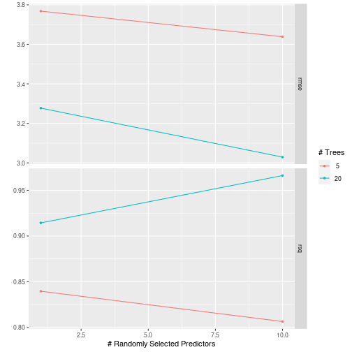
plot of chunk grid_search_tuning5
If you want to extract the actual grid used behind the scenes, pull_tflow_grid returns exactly that, after the model has been fitted.
res %>% pull_tflow_grid()
#> # A tibble: 4 x 2
#>    mtry trees
#>   <int> <int>
#> 1     1     5
#> 2    10     5
#> 3     1    20
#> 4    10    20
Once you’ve tuned your model you want to choose the final model. complete_tflow takes care of finding by the best combination of values for you. When you provide the metric of interest, it searches for the combination of parameters with the lowest error for your metric:
final_mod <- res %>% complete_tflow(metric = "rmse")

# Otherwise, you can provide the values manually yourself
# best <- data.frame(trees = 10, min_n = 20, mtry = 5)
# final_mod <- res %>% complete_tflow(best_params = best)

final_mod
#> ══ Tidyflow [trained] ══════════════════════════════════════════════════════════
#> Data: 32 rows x 11 columns
#> Split: initial_split w/ default args
#> Formula: mpg ~ .
#> Resample: vfold_cv w/ default args
#> Grid: grid_regular w/ trees = ~trees(range = c(5, 20)), levels = ~2
#> Model:
#> Random Forest Model Specification (regression)
#>
#> Main Arguments:
#>   mtry = 10
#>   trees = 20
#>   min_n = 20
#>
#> Computational engine: randomForest
#>
#> ══ Results ═════════════════════════════════════════════════════════════════════
#>
#> Tuning results:
#>
#> # A tibble: 5 x 4
#>   splits         id     .metrics         .notes
#>   <list>         <chr>  <list>           <list>
#> 1 <split [21/3]> Fold01 <tibble [8 × 6]> <tibble [0 × 1]>
#> 2 <split [21/3]> Fold02 <tibble [8 × 6]> <tibble [0 × 1]>
#> 3 <split [21/3]> Fold03 <tibble [8 × 6]> <tibble [0 × 1]>
#> 4 <split [21/3]> Fold04 <tibble [8 × 6]> <tibble [0 × 1]>
#> 5 <split [22/2]> Fold05 <tibble [8 × 6]> <tibble [0 × 1]>
#>
#> ... and 5 more lines.
#>
#>
#> Fitted model:
#>
#> Call:
#>  randomForest(x = as.data.frame(x), y = y, ntree = ~20L, mtry = ~10L,      nodesize = ~20)
#>                Type of random forest: regression
#>                      Number of trees: 20
#>
#> ...
#> and 4 more lines.
complete_tflow takes care of fitting the model with the best parameters on the entire training data. Now you can predict on the training or testing data automatically with predict_training or predict_testing.
final_mod %>%
  predict_training() %>%
  rsq(mpg, .pred)
#> # A tibble: 1 x 3
#>   .metric .estimator .estimate
#>   <chr>   <chr>          <dbl>
#> 1 rsq     standard       0.875
The tune package and tidymodels are very powerful tools for doing machine learning. In this vignette, I tried to extend their work by providing a unified interface for working with tune that uses the grid search framework bundled together with all the other common machine learning steps.
Want to see tidyflow and tune in action? The tidymodels team has a vignette showcasing how to use tune and tidymodels here. I’ve adapted their code to fully run within a tidyflow workflow. Here’s the replication code:
library(tidymodels)
library(tidyflow)
library(readr)       # for importing data
library(vip)         # for variable importance plots
library(readr)

hotels <-
  read_csv("https://tidymodels.org/start/case-study/hotels.csv") %>%
  mutate_if(is.character, as.factor)

lr_mod <- logistic_reg(penalty = tune(), mixture = 1) %>% set_engine("glmnet")

holidays <- c("AllSouls", "AshWednesday", "ChristmasEve", "Easter",
              "ChristmasDay", "GoodFriday", "NewYearsDay", "PalmSunday")

lr_recipe <-
  ~ .x %>%
    recipe(children ~ .) %>%
    step_date(arrival_date) %>%
    step_holiday(arrival_date, holidays = holidays) %>%
    step_rm(arrival_date) %>%
    step_dummy(all_nominal(), -all_outcomes()) %>%
    step_zv(all_predictors()) %>%
    step_normalize(all_predictors())

tflow <-
  hotels %>%
  tidyflow(seed = 123) %>%
  plug_split(initial_split, strata = "children") %>%
  plug_resample(validation_split, strata = "children", prop = 0.8) %>%
  plug_recipe(lr_recipe) %>%
  plug_grid(expand.grid, penalty = 10^seq(-4, -1, length.out = 30)) %>%
  plug_model(lr_mod)

cntrl <- control_tidyflow(control_grid = control_grid(save_pred = TRUE))
p_res <- tflow %>% fit(control = cntrl)

p_res %>%
  pull_tflow_fit_tuning() %>%
  collect_metrics() %>%
  filter(.metric == "roc_auc") %>%
  ggplot(aes(x = penalty, y = mean)) +
  geom_point() +
  geom_line() +
  ylab("Area under the ROC Curve") +
  scale_x_log10(labels = scales::label_number())

top_models <-
  p_res %>%
  pull_tflow_fit_tuning() %>%
  show_best("roc_auc", n = 15) %>%
  arrange(penalty)

lr_best <- top_models %>% slice(12)

lr_auc <-
  p_res %>%
  pull_tflow_fit_tuning() %>%
  collect_predictions(parameters = lr_best) %>%
  roc_curve(children, .pred_children) %>%
  mutate(model = "Logistic Regression")

autoplot(lr_auc)

# Let's run in parallel
cores <- parallel::detectCores() - 2

rf_mod <-
  rand_forest(mtry = tune(), min_n = tune(), trees = 1000) %>%
  set_engine("randomForest", num.threads = cores) %>%
  set_mode("classification")

rf_recipe <-
  ~ .x %>%
    recipe(children ~ .) %>%
    step_date(arrival_date) %>%
    step_holiday(arrival_date) %>%
    step_rm(arrival_date)

tflow <-
  tflow %>%
  replace_recipe(rf_recipe) %>%
  replace_model(rf_mod) %>%
  replace_grid(grid_latin_hypercube, size = 25)

rf_res <- tflow %>% fit(control = cntrl)

rf_res %>%
  pull_tflow_fit_tuning() %>%
  autoplot() +
  ylim(c(0.88, 0.93))

rf_best <-
  rf_res %>%
  pull_tflow_fit_tuning() %>%
  select_best(metric = "roc_auc")

rf_auc <-
  rf_res %>%
  pull_tflow_fit_tuning() %>%
  collect_predictions(parameters = rf_best) %>%
  roc_curve(children, .pred_children) %>%
  mutate(model = "Random Forest")

bind_rows(rf_auc, lr_auc) %>%
  ggplot(aes(x = 1 - specificity, y = sensitivity, col = model)) +
  geom_path(lwd = 1.5, alpha = 0.8) +
  geom_abline(lty = 3) +
  coord_equal() +
  scale_color_viridis_d(option = "plasma", end = .6)

final_res <-
  rf_res %>%
  complete_tflow(metric = "roc_auc")

final_res %>%
  predict_testing(type = "prob") %>%
  roc_curve(children, .pred_children) %>%
  autoplot()