This vignette aims to exemplify how you can use recipes within a tidyflow.
A tidyflow is a bundle of steps that allow you to bundle together your data, splitting, resampling, preprocessing, modeling, and grid search. For preprocessing your data, the tidymodels ecosystem contains the recipes package. This package allows to create very concise and clean pipelines of transforming your data. Let’s create a very simple recipe that takes the logarithm of the variable qsec:
rcp <-
mtcars %>%
recipe(mpg ~ .) %>%
step_log(qsec)
rcp
#> Data Recipe
#>
#> Inputs:
#>
#> role #variables
#> outcome 1
#> predictor 10
#>
#> Operations:
#>
#> Log transformation on qsecThe recipe contains the model formula (mpg ~ .) and a preprocessing step step_log(qsec). How do we incorporate this in our tidyflow? We use plug_recipe but we need to change this recipe to be a formula:
rcp <-
~ .x %>%
recipe(mpg ~ .) %>%
step_log(qsec)
tflow <-
mtcars %>%
tidyflow(seed = 5131) %>%
plug_recipe(rcp)
tflow
#> ══ Tidyflow ════════════════════════════════════════════════════════════════════
#> Data: 32 rows x 11 columns
#> Split: None
#> Recipe: available
#> Resample: None
#> Grid: None
#> Model: NoneDid you notice that we replace mtcars with .x and that .x has a ~ in front of it? Those are the only two things that changes from our previous recipe. tidyflow already knows that .x will be the placeholder for the data and will figure out where to place the recipe in the order of execution.
Having said this, there’s no need to specify a formula for the model definition: the recipe already contains this formula! So let’s split the data into training and testing and fit a linear regression:
tflow <-
tflow %>%
plug_split(initial_split) %>%
plug_model(linear_reg() %>% set_engine("lm"))
final_model <- tflow %>% fit()
final_model %>%
pull_tflow_fit()
#> parsnip model object
#>
#> Fit time: 5ms
#>
#> Call:
#> stats::lm(formula = ..y ~ ., data = data)
#>
#> Coefficients:
#> (Intercept) cyl disp hp drat wt
#> -35.739311 0.329900 0.003209 -0.015191 1.656429 -2.376667
#> qsec vs am gear carb
#> 19.316946 0.767142 3.789040 0.074718 -0.278102Defining your preprocessing steps in the recipe has several advantages among which are that the tidyflow takes care of applying these preprocessing steps in the training/testing data automatically. You can automatically predict on the training data and expect the tidyflow to calculate the log of qsec automatically:
final_model %>%
predict_training()
#> # A tibble: 24 x 12
#> mpg cyl disp hp drat wt qsec vs am gear carb .pred
#> <dbl> <dbl> <dbl> <dbl> <dbl> <dbl> <dbl> <dbl> <dbl> <dbl> <dbl> <dbl>
#> 1 21 6 160 110 3.9 2.62 16.5 0 1 4 4 22.4
#> 2 21 6 160 110 3.9 2.88 17.0 0 1 4 4 22.4
#> 3 21.4 6 258 110 3.08 3.22 19.4 1 0 3 1 20.9
#> 4 18.1 6 225 105 2.76 3.46 20.2 1 0 3 1 20.5
#> 5 14.3 8 360 245 3.21 3.57 15.8 0 0 3 4 13.6
#> 6 24.4 4 147. 62 3.69 3.19 20 1 0 4 2 22.0
#> 7 22.8 4 141. 95 3.92 3.15 22.9 1 0 4 2 24.6
#> 8 19.2 6 168. 123 3.92 3.44 18.3 1 0 4 4 19.3
#> 9 16.4 8 276. 180 3.07 4.07 17.4 0 0 3 3 15.0
#> 10 17.3 8 276. 180 3.07 3.73 17.6 0 0 3 3 16.1
#> # … with 14 more rowsNote that the qsec column here is untransformed but the model used to predict on the new .pred column was indeed logged. How can you be sure? You can extract the transformed training data with pull_tflow_training with prep = TRUE:
final_model %>%
pull_tflow_training(prep = TRUE)
#> mpg cyl disp hp drat wt qsec vs am gear carb
#> 1 21.0 6 160.0 110 3.90 2.620 2.800933 0 1 4 4
#> 2 21.0 6 160.0 110 3.90 2.875 2.834389 0 1 4 4
#> 3 21.4 6 258.0 110 3.08 3.215 2.967333 1 0 3 1
#> 4 18.1 6 225.0 105 2.76 3.460 3.006672 1 0 3 1
#> 5 14.3 8 360.0 245 3.21 3.570 2.762538 0 0 3 4
#> 6 24.4 4 146.7 62 3.69 3.190 2.995732 1 0 4 2
#> 7 22.8 4 140.8 95 3.92 3.150 3.131137 1 0 4 2
#> 8 19.2 6 167.6 123 3.92 3.440 2.906901 1 0 4 4
#> 9 16.4 8 275.8 180 3.07 4.070 2.856470 0 0 3 3
#> 10 17.3 8 275.8 180 3.07 3.730 2.867899 0 0 3 3
#> 11 15.2 8 275.8 180 3.07 3.780 2.890372 0 0 3 3
#> 12 10.4 8 472.0 205 2.93 5.250 2.889260 0 0 3 4
#> 13 14.7 8 440.0 230 3.23 5.345 2.857619 0 0 3 4
#> 14 32.4 4 78.7 66 4.08 2.200 2.968875 1 1 4 1
#> 15 33.9 4 71.1 65 4.22 1.835 2.990720 1 1 4 1
#> 16 21.5 4 120.1 97 3.70 2.465 2.996232 1 0 3 1
#> 17 15.5 8 318.0 150 2.76 3.520 2.825537 0 0 3 2
#> 18 15.2 8 304.0 150 3.15 3.435 2.850707 0 0 3 2
#> 19 19.2 8 400.0 175 3.08 3.845 2.836150 0 0 3 2
#> 20 27.3 4 79.0 66 4.08 1.935 2.939162 1 1 4 1
#> 21 15.8 8 351.0 264 4.22 3.170 2.674149 0 1 5 4
#> 22 19.7 6 145.0 175 3.62 2.770 2.740840 0 1 5 6
#> 23 15.0 8 301.0 335 3.54 3.570 2.681022 0 1 5 8
#> 24 21.4 4 121.0 109 4.11 2.780 2.923162 1 1 4 2One drawback from the print out of the tidyflow is that you can really see the type of preprocessing that was used for fitting the model. pull_tflow_prepped_recipe returns the fitted recipe on the final model and contains all the steps used in the recipe:
final_model %>%
pull_tflow_prepped_recipe()
#> Data Recipe
#>
#> Inputs:
#>
#> role #variables
#> outcome 1
#> predictor 10
#>
#> Training data contained 24 data points and no missing data.
#>
#> Operations:
#>
#> Log transformation on qsec [trained]Another advantage of a recipe preprocessing step is that it allows to perform a grid search on values defined in the preprocessing. For example, suppose we want to calculate the polynomial of sec. We could try qsec^2, qsec^3, etc… Until we find a polynomial that maximizes our predictive accuracy. Recipes accept an object called tune that signals that we will try many values for a particular argument (polynomials in this case). If you specify a plug_split, tidyflow can figure out some possible values to use are run the entire grid search for you. For example:
# New recipe that will try many values for degree
# degree here means the polynomial degree.
# For example, qsec^2, qsec^3, etc...
rcp <-
~ .x %>%
recipe(mpg ~ .) %>%
step_poly(qsec, degree = tune())
final_model <-
tflow %>% # Reuse the same tidyflow from before
replace_recipe(rcp) %>% # Replace the recipe with the new one
plug_resample(vfold_cv) %>% # Plug in the cross-validation for grid search
plug_grid(grid_regular) %>% # Plug in the type of grid search
fit()
final_model
#> ══ Tidyflow [tuned] ════════════════════════════════════════════════════════════
#> Data: 32 rows x 11 columns
#> Split: initial_split w/ default args
#> Recipe: available
#> Resample: vfold_cv w/ default args
#> Grid: grid_regular w/ default args
#> Model:
#> Linear Regression Model Specification (regression)
#>
#> Computational engine: lm
#>
#> ══ Results ═════════════════════════════════════════════════════════════════════
#>
#> Tuning results:
#>
#> # A tibble: 5 x 4
#> splits id .metrics .notes
#> <list> <chr> <list> <list>
#> 1 <split [21/3]> Fold01 <tibble [6 × 5]> <tibble [0 × 1]>
#> 2 <split [21/3]> Fold02 <tibble [6 × 5]> <tibble [0 × 1]>
#> 3 <split [21/3]> Fold03 <tibble [6 × 5]> <tibble [0 × 1]>
#> 4 <split [21/3]> Fold04 <tibble [6 × 5]> <tibble [0 × 1]>
#> 5 <split [22/2]> Fold05 <tibble [6 × 5]> <tibble [0 × 1]>
#>
#> ... and 5 more lines.The result is now a tuning grid and not a final model. As expected, this is because tidyflow already fit many models using different values for degree. We can explore the performance of the model with this model.
final_model %>%
pull_tflow_fit_tuning() %>%
autoplot()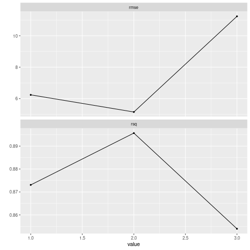
plot of chunk grid_search_recipe
The lowest error for both the \(RMSE\) and the \(R^2\) seems to be a model of degree = 2. We can specify this directly into complete_tflow or just allow complete_tflow to determine this for you:
# Manual approach
best_model <- final_model %>% complete_tflow(best_params = data.frame(degree = 2))
# Allow `complete_tflow` to determine this for you
best_model <- final_model %>% complete_tflow(metric = "rmse")
best_model %>%
predict_training()
#> # A tibble: 24 x 12
#> mpg cyl disp hp drat wt qsec vs am gear carb .pred
#> <dbl> <dbl> <dbl> <dbl> <dbl> <dbl> <dbl> <dbl> <dbl> <dbl> <dbl> <dbl>
#> 1 21 6 160 110 3.9 2.62 16.5 0 1 4 4 21.0
#> 2 21 6 160 110 3.9 2.88 17.0 0 1 4 4 22.0
#> 3 21.4 6 258 110 3.08 3.22 19.4 1 0 3 1 20.6
#> 4 18.1 6 225 105 2.76 3.46 20.2 1 0 3 1 19.2
#> 5 14.3 8 360 245 3.21 3.57 15.8 0 0 3 4 12.8
#> 6 24.4 4 147. 62 3.69 3.19 20 1 0 4 2 23.2
#> 7 22.8 4 141. 95 3.92 3.15 22.9 1 0 4 2 23.1
#> 8 19.2 6 168. 123 3.92 3.44 18.3 1 0 4 4 19.4
#> 9 16.4 8 276. 180 3.07 4.07 17.4 0 0 3 3 14.4
#> 10 17.3 8 276. 180 3.07 3.73 17.6 0 0 3 3 16.8
#> # … with 14 more rowsThe recipes package and tidymodels and very powerful tools for doing machine learning. In this vignette, I tried to extend their work by providing a unified interface for working with tidymodels that uses the recipe framework bundled together with all the other common machine learning steps.
Want to see tidyflow and recipes in action? The tidymodels team has a vignette showcasing how to use recipes and tidymodels here. I’ve adapted their code to fully run within a tidyflow workflow. Here’s the replication code:
library(tidymodels)
library(tidyflow)
library(nycflights13)
## Start initial preprocessing
flight_data <-
flights %>%
mutate(
# Convert the arrival delay to a factor
arr_delay = ifelse(arr_delay >= 30, "late", "on_time"),
arr_delay = factor(arr_delay),
# We will use the date (not date-time) in the recipe below
date = as.Date(time_hour)
) %>%
# Include the weather data
inner_join(weather, by = c("origin", "time_hour")) %>%
# Only retain the specific columns we will use
select(dep_time, flight, origin, dest, air_time, distance,
carrier, date, arr_delay, time_hour) %>%
# Exclude missing data
na.omit() %>%
# For creating models, it is better to have qualitative columns
# encoded as factors (instead of character strings)
mutate_if(is.character, as.factor)
## End initial preprocessing
# Model formula and recipe preprocessing
flight_rec <-
~ .x %>%
recipe(arr_delay ~ .) %>%
update_role(flight, time_hour, new_role = "ID") %>%
step_date(date, features = c("dow", "month")) %>%
step_holiday(date, holidays = timeDate::listHolidays("US")) %>%
step_rm(date) %>%
step_dummy(all_nominal(), -all_outcomes()) %>%
step_zv(all_predictors())
# tidyflow preparation with the recipe
tflow <-
flight_data %>%
tidyflow(seed = 555) %>%
plug_split(initial_split, prop = 3/4) %>%
plug_recipe(flight_rec) %>%
plug_model(logistic_reg() %>% set_engine("glm"))
# Fit final model
flights_fit <- fit(tflow)
# Predict on testing and evaluate a `roc_curve`
flights_fit %>%
predict_testing(type = "prob") %>%
roc_curve(truth = arr_delay, .pred_late) %>%
autoplot()