Multilevel modeling – Part 1
I’ve been reading Andrew Gelman’s and Jennifer Hill’s book again but this time concentrating on the multilevel section of the book. I finished the first chapter (chapter 12) and got fixed on the exercises 12.2, 12.3 and 12.4. I finally completed them and I thought I’d share the three exercises in two posts, mostly for me to come back to these in the future. The first exercise goes as follows:
Write a model predicting CD4 percentage as a function of time with varying intercepts across children. Fit using lmer() and interpret the coefficient for time.
Extend the model in (a) to include child-level predictors (that is, group-level predictors) for treatment and age at baseline. Fit using lmer() and interpret the coefficients on time, treatment, and age at baseline.
Investigate the change in partial pooling from (a) to (b) both graphically and numerically.
Compare results in (b) to those obtained in part (c).
The data set they’re referring is called ‘CD4’ and as they authors explain in the book it measures ‘… CD4 percentages for a set of young children with HIV who were measured several times over a period of two years. The dataset also includes the ages of the children at each measurement..’. I’m not sure what CD4 means, but that shouldn’t stop us from at least interpreting the results and answering the questions. Let’s start with the exercises:
- Write a model predicting CD4 percentage as a function of time with varying intercepts across children. Fit using lmer() and interpret the coefficient for time. The data argument is excluding some NA’s because the next model is to be compared with this model and we need to have the same number of observations
suppressWarnings(suppressMessages(library(arm)))
cd4 <- read.csv("http://www.stat.columbia.edu/~gelman/arm/examples/cd4/allvar.csv")

head(cd4)
## VISIT newpid VDATE CD4PCT arv visage treatmnt CD4CNT baseage
## 1 1 1 6/29/1988 18 0 3.910000 1 323 3.91
## 2 4 1 1/19/1989 37 0 4.468333 1 610 3.91
## 3 7 1 4/13/1989 13 0 4.698333 1 324 3.91
## 4 10 1 NA 0 5.005000 1 NA 3.91
## 5 13 1 11/30/1989 13 0 5.330833 1 626 3.91
## 6 16 1 NA NA NA 1 220 3.91# Let's transform the VDATE variable into date format
cd4$VDATE <- as.Date(cd4$VDATE, format = "%m/%d/%Y")
mod1 <- lmer(CD4PCT ~
VDATE +
(1 | newpid),
data = subset(cd4, !is.na(treatmnt) & !is.na(baseage)))
display(mod1)## lmer(formula = CD4PCT ~ VDATE + (1 | newpid), data = subset(cd4,
## !is.na(treatmnt) & !is.na(baseage)))
## coef.est coef.se
## (Intercept) 66.04 9.48
## VDATE -0.01 0.00
##
## Error terms:
## Groups Name Std.Dev.
## newpid (Intercept) 11.65
## Residual 7.31
## ---
## number of obs: 1072, groups: newpid, 250
## AIC = 7914, DIC = 7885.8
## deviance = 7895.9The time coefficient simply means that as time increases the percentage of CD4 decreases by 0.01 percent for each child. The effect size is really small, although significant. We can also see that most of the variation in CD4 is between children rather than within children (that is between time because that’s the variation within each child)
- Extend the model in (a) to include child-level predictors (that is, group-level predictors) for treatment and age at baseline. Fit using lmer() and interpret the coefficients on time, treatment, and age at baseline.
mod2 <- lmer(CD4PCT ~
               VDATE +
               treatmnt +
               baseage +
               (1 | newpid),
             data = cd4)

display(mod2)
## lmer(formula = CD4PCT ~ VDATE + treatmnt + baseage + (1 | newpid),
## data = cd4)
## coef.est coef.se
## (Intercept) 67.28 9.82
## VDATE -0.01 0.00
## treatmnt 1.26 1.54
## baseage -1.00 0.34
##
## Error terms:
## Groups Name Std.Dev.
## newpid (Intercept) 11.45
## Residual 7.32
## ---
## number of obs: 1072, groups: newpid, 250
## AIC = 7906.3, DIC = 7878.8
## deviance = 7886.5The time coefficients is exactly the same so neither the treatment or the base age is correlated with the date in which the students were measured. Those who were treated have on average about 1.26% more CD4 than the non-treated. And finally, children which were older at the base measure have about 1% less CD4 than younger children at base. The between-child variance went down from 11.65 to 11.45, so either treatment, baseage or both explained some of the differences between children. The within child variation is practically the same.
The next exercises uses a term called ‘partial pooling’. This term took me some time to understand but it basically means that we’re neither running a regression ignoring any multilevel structure (complete pooling of the groups) or running a regression for each group separately (complete no-pooling). Running a partially pooled model means being able to have single parameters (like in a completely-pooled model), but estimated from separate regression models for each group(like in a complete-no-pooled model).
How we can investigate the changes in partial pooling? A completely pooled model runs perfectly when you have little to no variation between groups. Whenever a set of predictors shrinks the between group variation, we’re getting closer to a model with less and less between group variation ( so completely pooled). How can we measure this? In our case, because we’re modeling a varying intercept, we can compare the confidence intervals of the intercept of each group intercept and see if the estimation has become more certain. Numerically, we can check whether the between group variation has decreased, becoming closer to a completely-pooled model.
- Investigate the change in partial pooling from (a) to (b) both graphically and numerically.
suppressMessages(suppressWarnings(library(ggplot2)))
# Change in standard errors

# First and second model intercepts
df1 <- coef(mod1)$newpid[,1 , drop = F]
df2 <- coef(mod2)$newpid[,1 , drop = F]
names(df1) <- c("int")
names(df2) <- c("int")

# Confidence intervals for each intercept for both moels
df1$ci_bottom <- df1$int + (-2 * se.ranef(mod1)$newpid[,1])
df1$ci_upper <- df1$int + (2 * se.ranef(mod1)$newpid[,1])

df2$ci_bottom <- df2$int + (-2 * se.ranef(mod2)$newpid[,1])
df2$ci_upper <- df2$int + (2 * se.ranef(mod2)$newpid[,1])

# Now we need to compare whether the CI's shrunk from
# the first to the second model

# Calculate difference
df1$diff <- df1$ci_upper - df1$ci_bottom
df2$dff <- df2$ci_upper - df2$ci_bottom

# Create a df with both differences
df3 <- data.frame(cbind(df1$diff, df2$dff))

# Create a difference out of that
df3$diff <- df3$X1 - df3$X2

# Graph it
ggplot(df3, aes(diff)) + geom_histogram(bins = 100) +
  xlim(0, 0.2)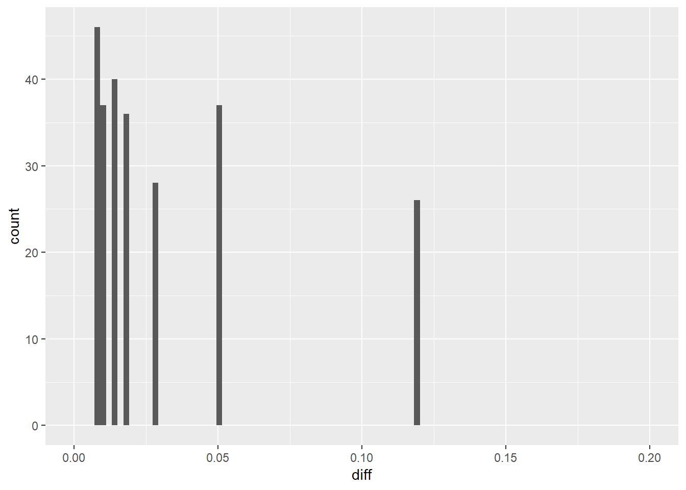
It looks like the difference is always higher than zero which means that in the second model the difference between the upper and lower CI is smaller than in the first model. This suggests we have greater certainty of our estimation by including the two predictors in the model.
# Numerically, the between-child variance in the first
# model was:
display(mod1)
## lmer(formula = CD4PCT ~ VDATE + (1 | newpid), data = subset(cd4,
## !is.na(treatmnt) & !is.na(baseage)))
## coef.est coef.se
## (Intercept) 66.04 9.48
## VDATE -0.01 0.00
##
## Error terms:
## Groups Name Std.Dev.
## newpid (Intercept) 11.65
## Residual 7.31
## ---
## number of obs: 1072, groups: newpid, 250
## AIC = 7914, DIC = 7885.8
## deviance = 7895.911.65 / (11.65 + 7.31)## [1] 0.6144515# For the second model
display(mod2)## lmer(formula = CD4PCT ~ VDATE + treatmnt + baseage + (1 | newpid),
## data = cd4)
## coef.est coef.se
## (Intercept) 67.28 9.82
## VDATE -0.01 0.00
## treatmnt 1.26 1.54
## baseage -1.00 0.34
##
## Error terms:
## Groups Name Std.Dev.
## newpid (Intercept) 11.45
## Residual 7.32
## ---
## number of obs: 1072, groups: newpid, 250
## AIC = 7906.3, DIC = 7878.8
## deviance = 7886.511.45 / (11.45 + 7.32)## [1] 0.610016The between variance went down JUST a little, in line with the tiny reduction in the standard errors of the intercept.
The last question asks:
Compare results in (b) to those obtained in part (c).
It looks like from the results in (c) the second model a bit more certain in making estimations because it shrinks the partial pooling closer to complete-pooling. As Gelman and Hill explain in page 270, multilevel modeling is most effective when closest to complete-pooling because the estimation of individual group parameters can be done much more precisely, specially for groups with a small amount of observations.
In the next post we’ll cover exercises 12.3 and 12.4 which build on the models outlined here.