Multilevel modeling – Part 2
This is a continuation of the multilevel exercise 12.2 from chapter 12 of Data Analysis Using Regression and Multilevel/Hierarchical Models. In the last post (link to previous post) we explored the basic interpretation of multilevel modeling with a varying intercept and delved into comparing models and understanding partial pooling.
This was all done by completing the exercise 12.2 from chapter 12 of the book Data Analysis Using Regression and Multilevel/Hierarchical Models. Exercises 12.3 and 12.4 continue using the same dataset and the same models, so I figured I’d post them here. Let’s start.
Exercise 12.3 asks:
- Predictions for new observations and new groups:
Use the model fit from Exercise 12.2 (b) to generate simulation of predicted CD4 percentages for each child in the dataset at a hypothetical next time point.
Use the same model fit to generate simulations of CD4 percentages at each of the time periods for a new child who was 4 years old at baseline.
Let’s start:
suppressWarnings(suppressMessages(library(arm)))
cd4 <- read.csv("http://www.stat.columbia.edu/~gelman/arm/examples/cd4/allvar.csv")

# Let's recreate the model from 12.2 (b)
cd4$VDATE <- as.Date(cd4$VDATE, format = "%m/%d/%Y")
mod2 <- lmer(CD4PCT ~ VDATE + treatmnt + baseage + (1 | newpid), data = cd4)- Use the model fit from Exercise 12.2 (b) to generate simulation of predicted CD4 percentages for each child in the dataset at a hypothetical next time point.
For this we have to create a hypothetical next time point. Let’s choose:
pred_data <- subset(cd4, !is.na(treatmnt) & !is.na(baseage))
pred_data$VDATE <- as.Date("1989-01-01")


# Let's select only the independent variables from the model
pred_data <- pred_data[, -c(1, 4, 5, 6, 8)]

# Now we have a dataset with a fixed new date for each child
# but with the original values for all other variables.

# Let's estimate the predicted CD4 percentage for each child:
newpred <- predict(mod2, newdata = pred_data)

# That it! We have the predicted percentage of CD4 for a fixed date for every child.
# Let's look at the distribution
hist(newpred)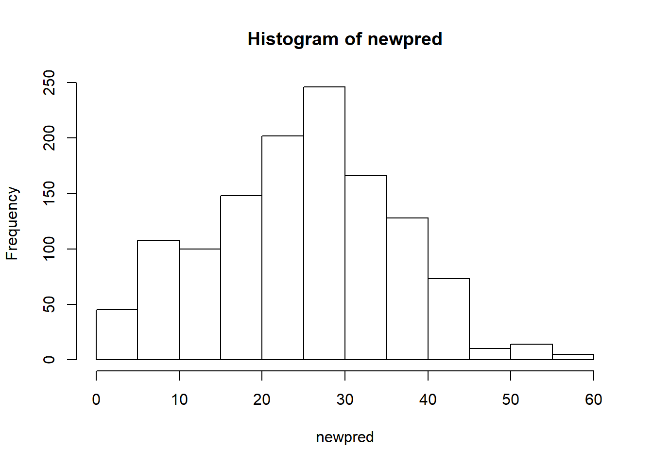
There’s quite some variation going from 0% to even 60%. It’d be nice to know what CD4 is.
Question (b) is pretty similar but instead of asking for a new time point for each child, it asks to predict the CD4 percentage for a new child who was 4 years old at the baseline with a set of hypothetical time periods.
- Use the same model fit to generate simulations of CD4 percentages at each of the time periods for a new child who was 4 years old at baseline.
For that we have to first create the dataset with the hypothetical child:
# I'll assume 7 hypothetical dates
hyp_child <- data.frame(newpid = 120,
                        VDATE = sample(cd4$VDATE[!is.na(cd4$VDATE)], 7),
                        baseage = 4,
                        treatmnt = 1)
The exercise doesn’t say anything about the treatment variable but I have to assign a value to it because it’s present in the previous model. I’ll assume this new child was in the treatment.
year_pred <- predict(mod2, newdata = hyp_child)That’s it! Now we have the predicted CD4 percentage for different time points for a hypothetical child.
Finally, exercise 12.4 posits this question:
Posterior predictive checking: continuing the previous exercise, use the fitted model from Exercise 12.2 (b) to simulate a new dataset of CD4 percentages (with the same sample size and ages of the original dataset) for the final time point of the study, and record the average CD4 percentage in this sample. Repeat this process 1000 times and compare the simulated distribution to the observed CD4 percentage at the final time point for the actual data.
This problem was a bit confusing because I don’t understand what they mean by the ‘final time point of the study’. Is it the last date in the VDATE variable? But that couldn’t be it because the sample size would be 1. I think what they mean is to take the original data and replace the VDATE variable with the final date available. Predict CD4 percentages for each child with this date (using the original ages of the data set) and calculate the mean of these predictions. After that, do the 1000 replications and compare the distribution with the actual CD4 percentage of the specific date. Let’s start.
# Make the data similar to the model in mod2
finaltime_data <- subset(cd4, !is.na(treatmnt) & !is.na(baseage))

# Assign the final date to the date variable
finaltime_data$VDATE <- as.Date(max(finaltime_data$VDATE, na.rm = T))

# Only select the variables present in the model
finaltime_data <- finaltime_data[, -c(1, 4, 5, 6, 8)]

# Calculate the mean predicted CD4 percentage and it's standard deviation
mean_cd4 <- mean(predict(mod2, newdata = finaltime_data), na.rm = T)
sd_cd4 <- sd(predict(mod2, newdata = finaltime_data), na.rm = T)

# Simulate 1000 observations considering the uncertainty
# and look at the distribution.
set.seed(421)

hist(rnorm(1000, mean_cd4, sd = sd_cd4))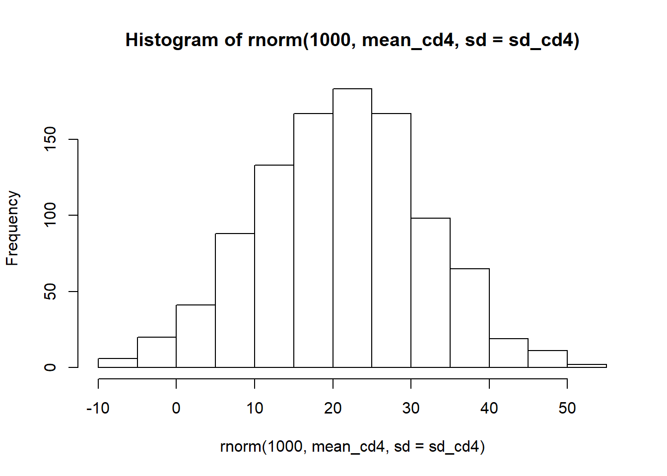
It’s incredibly wide and it even includes negative numbers, something impossible with percentages. But whats the actual CD4 percentage of that date?
cd4 <- subset(cd4, !is.na(VDATE))
cd4[cd4$VDATE == max(cd4$VDATE, na.rm = T), ]
## VISIT newpid VDATE CD4PCT arv visage treatmnt CD4CNT baseage
## 483 16 99 1991-01-14 39.0 1 1.497500 2 526 0.347500
## 1208 19 237 1991-01-14 21.2 0 2.510833 2 1036 1.073333And the mean is:
mean(c(39.0, 21.2))## [1] 30.1So our predictions are extremely uncertain. Over half our simulations are underestimating the date and a handful are overestimating the results. It looks like our model is terrible at predicting that final time point.
Well that’s it. Hope you enjoyed it. I’ll be completing more exercises in the future so remember to check back. ```