Web Scraping
Jorge Cimentada
A primer on webscraping

Primer on webscraping
Skip the usual ‘basics’ right into coding
Webscraping is the subtle art of being a ninja
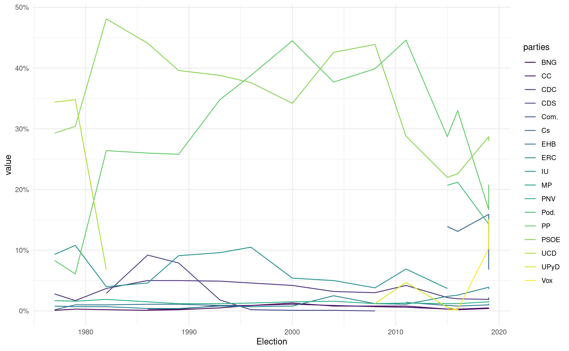
The plot above shows the election results for all political parties in Spain since 1978, all completely scraped from Wikipedia.
Chapter 2 from book
Scrapex
Webscraping tutorials are doomed to change
API examples are doomed to change
Predictability is important
scrapex is an R package with completely self-standing web scraping/API examples for eternity
Getting website data into R
library(scrapex)
library(rvest)
library(httr)
library(dplyr)
library(tidyr)
library(stringr)
library(ggplot2)

link <- history_elections_spain_ex()
link
[1] "/home/runner/.local/share/renv/cache/v5/R-4.2/x86_64-pc-linux-gnu/scrapex/0.0.1.9999/9aa78cbb3eccaaa811756b4bf07fdd1a/scrapex/extdata/history_elections_spain//Elections_Spain.html"Getting website data into R

Getting website data into R
Ethical web scraping is identifying yourself
Where can you find it?

Getting website data into R
{html_document}
<html class="client-nojs" lang="en" dir="ltr">
[1] <head>\n<meta http-equiv="Content-Type" content="text/html; charset=UTF-8 ...
[2] <body class="mediawiki ltr sitedir-ltr mw-hide-empty-elt ns-0 ns-subject  ...
Difficult to read – raw HTML code
Often too long to actually explore it
This output is mostly to confirm it was read and the header of the HTML file
Getting website data into R
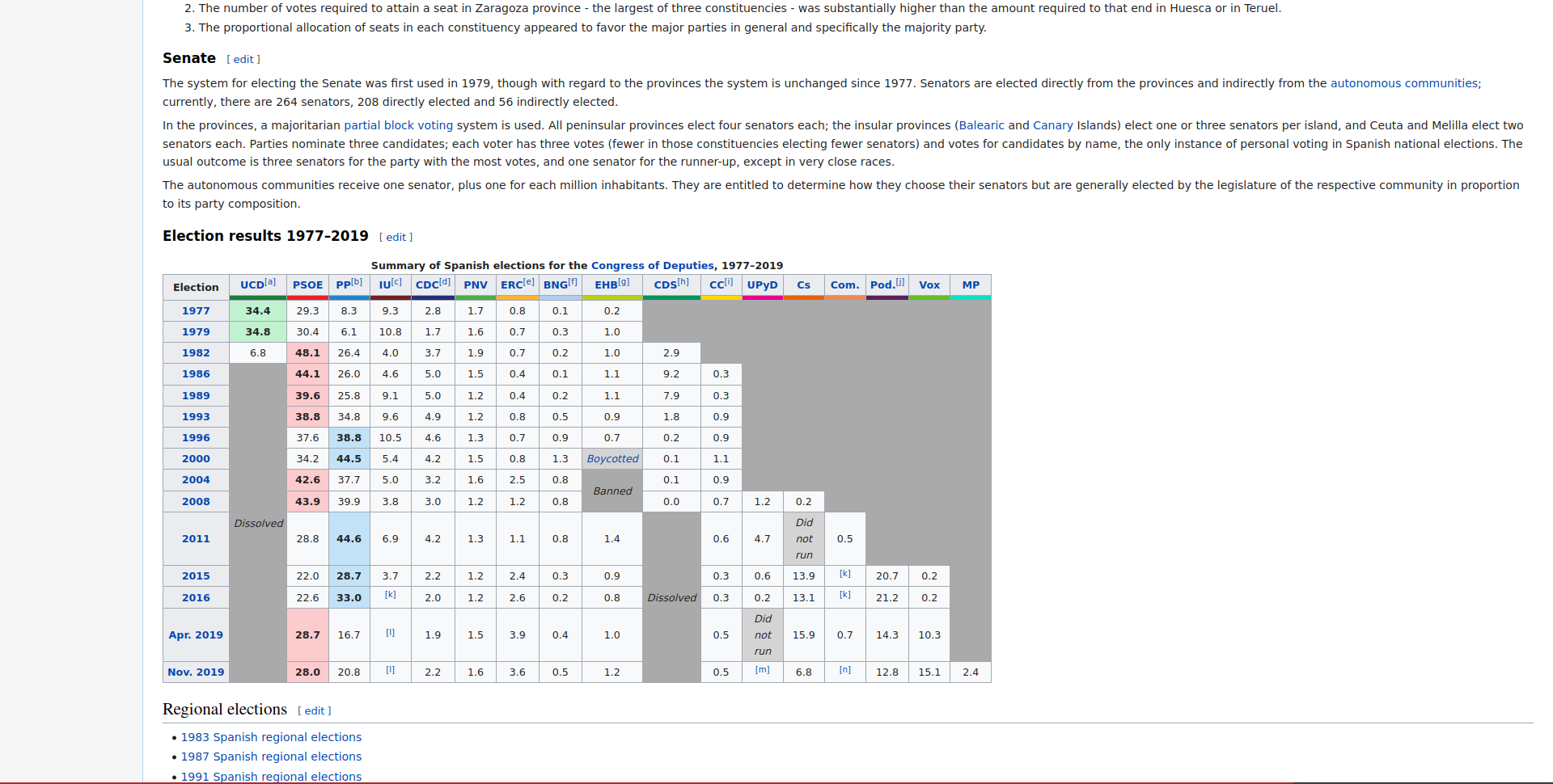
What we actually want:

Getting website data into R
The output from
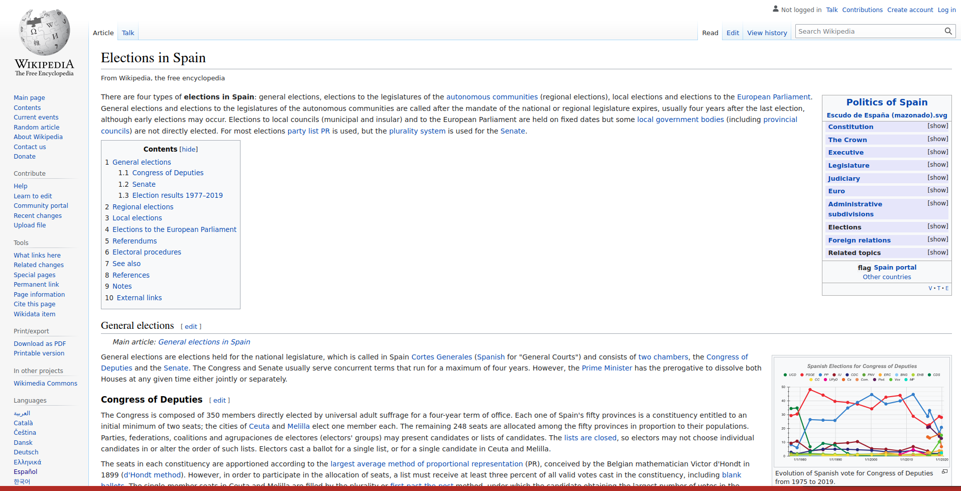
read_html()is difficult to understandGoal is to find actual election data on the website
rvestpackage hashtml_table()function that can extract tables from website and import into R.
Getting website data into R
Grabs all tables
We only pick the one we’re interested in.
# A tibble: 16 × 18
   Election  `UCD[a]`     PSOE `PP[b]` `IU[c]` `CDC[d]`   PNV `ERC[e]` `BNG[f]`
   <chr>     <chr>       <dbl>   <dbl> <chr>      <dbl> <dbl>    <dbl>    <dbl>
 1 Election  ""           NA      NA   ""          NA    NA       NA       NA
 2 1977      "34.4"       29.3     8.3 "9.3"        2.8   1.7      0.8      0.1
 3 1979      "34.8"       30.4     6.1 "10.8"       1.7   1.6      0.7      0.3
 4 1982      "6.8"        48.1    26.4 "4.0"        3.7   1.9      0.7      0.2
 5 1986      "Dissolved"  44.1    26   "4.6"        5     1.5      0.4      0.1
 6 1989      "Dissolved"  39.6    25.8 "9.1"        5     1.2      0.4      0.2
 7 1993      "Dissolved"  38.8    34.8 "9.6"        4.9   1.2      0.8      0.5
 8 1996      "Dissolved"  37.6    38.8 "10.5"       4.6   1.3      0.7      0.9
 9 2000      "Dissolved"  34.2    44.5 "5.4"        4.2   1.5      0.8      1.3
10 2004      "Dissolved"  42.6    37.7 "5.0"        3.2   1.6      2.5      0.8
11 2008      "Dissolved"  43.9    39.9 "3.8"        3     1.2      1.2      0.8
12 2011      "Dissolved"  28.8    44.6 "6.9"        4.2   1.3      1.1      0.8
13 2015      "Dissolved"  22      28.7 "3.7"        2.2   1.2      2.4      0.3
14 2016      "Dissolved"  22.6    33   "[k]"        2     1.2      2.6      0.2
15 Apr. 2019 "Dissolved"  28.7    16.7 "[l]"        1.9   1.5      3.9      0.4
16 Nov. 2019 "Dissolved"  28      20.8 "[l]"        2.2   1.6      3.6      0.5
# … with 9 more variables: `EHB[g]` <chr>, `CDS[h]` <chr>, `CC[i]` <dbl>,
#   UPyD <chr>, Cs <chr>, Com. <chr>, `Pod.[j]` <dbl>, Vox <dbl>, MP <dbl>
Data cleaning
- The first row is empty
- The “Election” column is a character column and contains string values
- Columns contain values which are not numbers
- Column names also have footnote values
The process of web scraping requires knowledge of regular expressions and data cleaning techniques.
Data cleaning
# A tibble: 16 × 8
   Election  `UCD[a]`    `IU[c]` `EHB[g]`    `CDS[h]`    UPyD        Cs    Com.
   <chr>     <chr>       <chr>   <chr>       <chr>       <chr>       <chr> <chr>
 1 Election  ""          ""      ""          ""          ""          ""    ""
 2 1977      "34.4"      "9.3"   "0.2"       ""          ""          ""    ""
 3 1979      "34.8"      "10.8"  "1.0"       ""          ""          ""    ""
 4 1982      "6.8"       "4.0"   "1.0"       "2.9"       ""          ""    ""
 5 1986      "Dissolved" "4.6"   "1.1"       "9.2"       ""          ""    ""
 6 1989      "Dissolved" "9.1"   "1.1"       "7.9"       ""          ""    ""
 7 1993      "Dissolved" "9.6"   "0.9"       "1.8"       ""          ""    ""
 8 1996      "Dissolved" "10.5"  "0.7"       "0.2"       ""          ""    ""
 9 2000      "Dissolved" "5.4"   "Boycotted" "0.1"       ""          ""    ""
10 2004      "Dissolved" "5.0"   "Banned"    "0.1"       ""          ""    ""
11 2008      "Dissolved" "3.8"   "Banned"    "0.0"       "1.2"       "0.2" ""
12 2011      "Dissolved" "6.9"   "1.4"       "Dissolved" "4.7"       "Did… "0.5"
13 2015      "Dissolved" "3.7"   "0.9"       "Dissolved" "0.6"       "13.… "[k]"
14 2016      "Dissolved" "[k]"   "0.8"       "Dissolved" "0.2"       "13.… "[k]"
15 Apr. 2019 "Dissolved" "[l]"   "1.0"       "Dissolved" "Did not r… "15.… "0.7"
16 Nov. 2019 "Dissolved" "[l]"   "1.2"       "Dissolved" "[m]"       "6.8" "[n]"
Data cleaning
- Build regular expression to replace all unwanted parts of the string
Data cleaning
- Replace the regex using
str_replace_all
semi_cleaned_data <-
  elections_data %>%
  mutate_if(
    is.character,
    ~ str_replace_all(string = .x, pattern = wrong_labels, replacement = NA_character_)
  )

semi_cleaned_data %>% select_if(is.character)
# A tibble: 16 × 8
Election `UCD[a]` `IU[c]` `EHB[g]` `CDS[h]` UPyD Cs Com.
<chr> <chr> <chr> <chr> <chr> <chr> <chr> <chr>
1 <NA> "" "" "" "" "" "" ""
2 1977 "34.4" "9.3" "0.2" "" "" "" ""
3 1979 "34.8" "10.8" "1.0" "" "" "" ""
4 1982 "6.8" "4.0" "1.0" "2.9" "" "" ""
5 1986 <NA> "4.6" "1.1" "9.2" "" "" ""
6 1989 <NA> "9.1" "1.1" "7.9" "" "" ""
7 1993 <NA> "9.6" "0.9" "1.8" "" "" ""
8 1996 <NA> "10.5" "0.7" "0.2" "" "" ""
9 2000 <NA> "5.4" <NA> "0.1" "" "" ""
10 2004 <NA> "5.0" <NA> "0.1" "" "" ""
11 2008 <NA> "3.8" <NA> "0.0" "1.2" "0.2" ""
12 2011 <NA> "6.9" "1.4" <NA> "4.7" <NA> "0.5"
13 2015 <NA> "3.7" "0.9" <NA> "0.6" "13.9" <NA>
14 2016 <NA> <NA> "0.8" <NA> "0.2" "13.1" <NA>
15 Apr. 2019 <NA> <NA> "1.0" <NA> <NA> "15.9" "0.7"
16 Nov. 2019 <NA> <NA> "1.2" <NA> <NA> "6.8" <NA>Data cleaning
Replace extra patterns of months
We replace again here because we want to replace with
""instead ofNA
semi_cleaned_data <-
  semi_cleaned_data %>%
  mutate(
    Election = str_replace_all(string = Election, pattern = "Apr. |Nov. ", replacement = "")
  )

semi_cleaned_data %>% select_if(is.character)
# A tibble: 16 × 8
Election `UCD[a]` `IU[c]` `EHB[g]` `CDS[h]` UPyD Cs Com.
<chr> <chr> <chr> <chr> <chr> <chr> <chr> <chr>
1 <NA> "" "" "" "" "" "" ""
2 1977 "34.4" "9.3" "0.2" "" "" "" ""
3 1979 "34.8" "10.8" "1.0" "" "" "" ""
4 1982 "6.8" "4.0" "1.0" "2.9" "" "" ""
5 1986 <NA> "4.6" "1.1" "9.2" "" "" ""
6 1989 <NA> "9.1" "1.1" "7.9" "" "" ""
7 1993 <NA> "9.6" "0.9" "1.8" "" "" ""
8 1996 <NA> "10.5" "0.7" "0.2" "" "" ""
9 2000 <NA> "5.4" <NA> "0.1" "" "" ""
10 2004 <NA> "5.0" <NA> "0.1" "" "" ""
11 2008 <NA> "3.8" <NA> "0.0" "1.2" "0.2" ""
12 2011 <NA> "6.9" "1.4" <NA> "4.7" <NA> "0.5"
13 2015 <NA> "3.7" "0.9" <NA> "0.6" "13.9" <NA>
14 2016 <NA> <NA> "0.8" <NA> "0.2" "13.1" <NA>
15 2019 <NA> <NA> "1.0" <NA> <NA> "15.9" "0.7"
16 2019 <NA> <NA> "1.2" <NA> <NA> "6.8" <NA>Data cleaning
- Remove first row
semi_cleaned_data <-
  semi_cleaned_data %>%
  mutate_all(as.numeric) %>%
  filter(!is.na(Election))

semi_cleaned_data
# A tibble: 15 × 18
Election `UCD[a]` PSOE `PP[b]` `IU[c]` `CDC[d]` PNV `ERC[e]` `BNG[f]`
<dbl> <dbl> <dbl> <dbl> <dbl> <dbl> <dbl> <dbl> <dbl>
1 1977 34.4 29.3 8.3 9.3 2.8 1.7 0.8 0.1
2 1979 34.8 30.4 6.1 10.8 1.7 1.6 0.7 0.3
3 1982 6.8 48.1 26.4 4 3.7 1.9 0.7 0.2
4 1986 NA 44.1 26 4.6 5 1.5 0.4 0.1
5 1989 NA 39.6 25.8 9.1 5 1.2 0.4 0.2
6 1993 NA 38.8 34.8 9.6 4.9 1.2 0.8 0.5
7 1996 NA 37.6 38.8 10.5 4.6 1.3 0.7 0.9
8 2000 NA 34.2 44.5 5.4 4.2 1.5 0.8 1.3
9 2004 NA 42.6 37.7 5 3.2 1.6 2.5 0.8
10 2008 NA 43.9 39.9 3.8 3 1.2 1.2 0.8
11 2011 NA 28.8 44.6 6.9 4.2 1.3 1.1 0.8
12 2015 NA 22 28.7 3.7 2.2 1.2 2.4 0.3
13 2016 NA 22.6 33 NA 2 1.2 2.6 0.2
14 2019 NA 28.7 16.7 NA 1.9 1.5 3.9 0.4
15 2019 NA 28 20.8 NA 2.2 1.6 3.6 0.5
# … with 9 more variables: `EHB[g]` <dbl>, `CDS[h]` <dbl>, `CC[i]` <dbl>,
# UPyD <dbl>, Cs <dbl>, Com. <dbl>, `Pod.[j]` <dbl>, Vox <dbl>, MP <dbl>Data cleaning
- Clean up column names
semi_cleaned_data <-
  semi_cleaned_data %>%
  rename_all(~ str_replace_all(.x, "\\[.+\\]", ""))

semi_cleaned_data
# A tibble: 15 × 18
Election UCD PSOE PP IU CDC PNV ERC BNG EHB CDS CC
<dbl> <dbl> <dbl> <dbl> <dbl> <dbl> <dbl> <dbl> <dbl> <dbl> <dbl> <dbl>
1 1977 34.4 29.3 8.3 9.3 2.8 1.7 0.8 0.1 0.2 NA NA
2 1979 34.8 30.4 6.1 10.8 1.7 1.6 0.7 0.3 1 NA NA
3 1982 6.8 48.1 26.4 4 3.7 1.9 0.7 0.2 1 2.9 NA
4 1986 NA 44.1 26 4.6 5 1.5 0.4 0.1 1.1 9.2 0.3
5 1989 NA 39.6 25.8 9.1 5 1.2 0.4 0.2 1.1 7.9 0.3
6 1993 NA 38.8 34.8 9.6 4.9 1.2 0.8 0.5 0.9 1.8 0.9
7 1996 NA 37.6 38.8 10.5 4.6 1.3 0.7 0.9 0.7 0.2 0.9
8 2000 NA 34.2 44.5 5.4 4.2 1.5 0.8 1.3 NA 0.1 1.1
9 2004 NA 42.6 37.7 5 3.2 1.6 2.5 0.8 NA 0.1 0.9
10 2008 NA 43.9 39.9 3.8 3 1.2 1.2 0.8 NA 0 0.7
11 2011 NA 28.8 44.6 6.9 4.2 1.3 1.1 0.8 1.4 NA 0.6
12 2015 NA 22 28.7 3.7 2.2 1.2 2.4 0.3 0.9 NA 0.3
13 2016 NA 22.6 33 NA 2 1.2 2.6 0.2 0.8 NA 0.3
14 2019 NA 28.7 16.7 NA 1.9 1.5 3.9 0.4 1 NA 0.5
15 2019 NA 28 20.8 NA 2.2 1.6 3.6 0.5 1.2 NA 0.5
# … with 6 more variables: UPyD <dbl>, Cs <dbl>, Com. <dbl>, Pod. <dbl>,
# Vox <dbl>, MP <dbl>Data cleaning
# Pivot from wide to long to plot it in ggplot
cleaned_data <-
  semi_cleaned_data %>%
  pivot_longer(-Election, names_to = "parties")

# Plot it
cleaned_data %>%
  ggplot(aes(Election, value, color = parties)) +
  geom_line() +
  scale_y_continuous(labels = function(x) paste0(x, "%")) +
  scale_color_viridis_d() +
  theme_minimal()
Data cleaning
