What time should I ride my bike?
For a few months now I’ve started developing a project on which I download live bicycle usage from the API of Bicing, the public bicycle service from the city of Barcelona. Before I started analyzing the data I wanted to harvest a reasonable amount of data to be able to get a representative sample of bicycle usage.
The first thing I did was to set up my Virtual Private Server (VPS) and set a
cronjob to email me every day after the scraping of the data is done. Check out a detailed tutorial on how to this hereThe second thing I did was to set up a MySQL database in my VPS and develop a program that interacts with the Barcelona Public Bicycle System API and feeds the database on a daily basis. Check out a detailed tutorial on how I did it here
I left this program grabing biclycle data of a station close to my house only in the mornings and evenings (moments I used the bicycle) for the last 3 months. This is my first attempt to analyze this data. Please take this as a work in progress as I develop more fine-grained understanding of the data.
Here I load the libraries and connect to the database in my VPS. Note how I hide the IP of the server and the password by grabbing it as environment variables.
library(DBI)
library(RMySQL)
library(caret)
library(viridis)
library(tidyverse)


password <- Sys.getenv("password")
host <- Sys.getenv("host")

con <- dbConnect(MySQL(),
                 dbname = "bicing", # in "" quotes
                 user = "cimentadaj", # in "" quotes
                 password = password,
                 host = host) # ip of my server
Next, let’s grab the data with a simple query. Let’s get some columns:
slotsis the number of available slots in the stationbikesis the number of available bikes in the station
These two columns are exact opposites. If the station can hold 20 bicycles and there are 8 slots available, then there’s 12 bicycles availables.
statusis the status of the station. WhetherOPNorCLOSED.timeis the specific date/time at which that row was returned from the API.
There’s an additional column named error_msg that has the error message if the API couldn’t retrieve the data. Let’s use only those which were scraped correctly. Let’s write that query and grab the data.
query <-
"SELECT slots, bikes, status, time
 FROM bicing_station
 WHERE hour(time) IN ('7', '8', '9', '10', '18', '19', '20')
 AND error_msg IS NULL;"

bicing <-
  dbGetQuery(con, query) %>%
  as_tibble() %>%
  mutate(time = lubridate::ymd_hms(time),
         slots = as.numeric(slots),
         bikes = as.numeric(slots))
Awesome. Now we have our data set.
bicing## # A tibble: 46,399 x 4
## slots bikes status time
## <dbl> <dbl> <chr> <dttm>
## 1 10. 10. OPN 2017-12-11 08:01:16
## 2 10. 10. OPN 2017-12-11 08:02:12
## 3 10. 10. OPN 2017-12-11 08:03:04
## 4 10. 10. OPN 2017-12-11 08:04:04
## 5 10. 10. OPN 2017-12-11 08:05:04
## 6 9. 9. OPN 2017-12-11 08:06:04
## 7 8. 8. OPN 2017-12-11 08:07:04
## 8 8. 8. OPN 2017-12-11 08:08:05
## 9 7. 7. OPN 2017-12-11 08:09:04
## 10 8. 8. OPN 2017-12-11 08:10:04
## # ... with 46,389 more rowsLet’s check if there’s any cases in which the station was not open.
bicing %>%
  filter(status != "OPN")
## # A tibble: 0 x 4
## # ... with 4 variables: slots <dbl>, bikes <dbl>, status <chr>,
## # time <dttm>Empty rows, alright, station has worked fine.
Let’s explore the number of bikes comparing between mornings/evenings
summary_time <-
  bicing %>%
  group_by(hour = as.factor(lubridate::hour(time))) %>%
  summarize(Average = mean(bikes, na.rm = TRUE),
            Median = median(bikes, na.rm = TRUE)) %>%
  gather(type, value, -hour)

bicing %>%
  mutate(hour = as.factor(lubridate::hour(time))) %>%
  ggplot(aes(hour, bikes)) +
  geom_jitter(alpha = 1/8) +
  geom_point(data = summary_time,
             aes(y = value, colour = type), size = 3) +
  theme_bw() +
  labs(x = "Hour of the day (24H)",
       y = "# of available bikes",
       title = "Mornings have greater bicycle usage than evenings",
       subtitle = "But number of bikes can vary betwen 0 and 20 in the morning") +
  scale_colour_manual(name = "Types", values = c('Average' = 'red', 'Median' = 'blue'))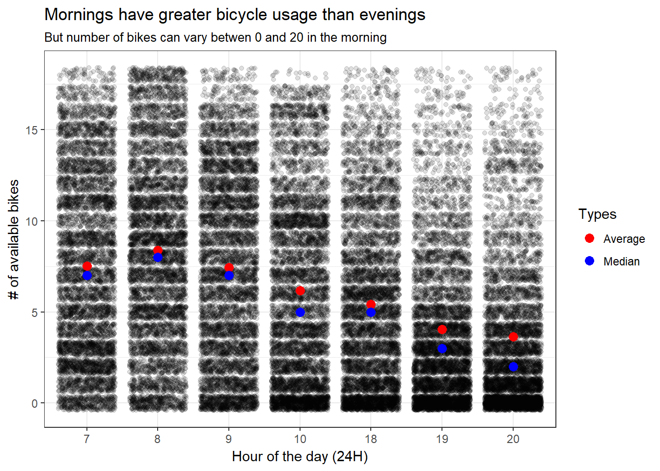
This is a bit revealing. Some take aways:
Mornings have greater number of bikes but they also have high variability. For example, look at the 8 AM category. Even though the average is at around 7 bikes, it’s also very likely that there’s 0 bikes as well as 20 bikes.
As time passes, more outliers appear in the distribution. We can infer this both from the overall distribution and the average and the mean are farther away from each other.
This is probably related to how Bicing fills out the stations (a few times a days a truck with bicycles passes by the station and fills them out). I think this is beginning to tell a story although perhaps it’s too early: usage in the mornings is heavy and very dynamic but as the day passes by more a more bikes are taken (either by the Bicing team or by citizens).
This gives no clear clue to the layman citizen: if it’s 8 AM, how likely am I find bikes? Let’s inspect further.
Logically, the next question is: does this differ by day of the week? Bloew I plot the average number of bikes per day/hour combination. In addition we’d also want to plot some sort of uncertainty indicator like the standard deviation. However, because it’s very common for bikes to be close to 7-10 bikes as average and below, I plot the uncertainty as the percentage of times that the station has over 10 bikes.
summary_time <-
  bicing %>%
  group_by(hour = as.factor(lubridate::hour(time)),
           day = as.factor(lubridate::wday(time, label = TRUE, week_start = TRUE))) %>%
  summarize(Average = mean(bikes, na.rm = TRUE),
            Variation = mean(bikes > 10, na.rm = TRUE)) %>%
  gather(type, value, -hour, -day)

p1 <-
  summary_time %>%
  filter(type == "Average") %>%
  ggplot(aes(hour, day, fill = value)) +
  geom_tile() +
  scale_fill_viridis(name = "Avg # of bikes") +
  labs(x = 'Hour of the day (24H)',
       y = 'Day of the week',
       title = 'Average number of bikes has a workin week/end of week divide',
       subtitle = 'Thu and Wed seem to have high peaks at 8, Sun and Sat have peaks at 10')

p2 <-
  summary_time %>%
  filter(type == "Variation") %>%
  ggplot(aes(hour, day, fill = value)) +
  geom_tile() +
  scale_fill_viridis(name = '% of times \n station has > 10 bikes') +
  labs(x = 'Hour of the day (24H)',
       y = 'Day of the week',
       title = 'Variability reflects same pattern as average # of bikes',
       subtitle = 'Thu and Wed seem to have > 10 bikes often at 8, Sun and Sat have peaks at 10')

p1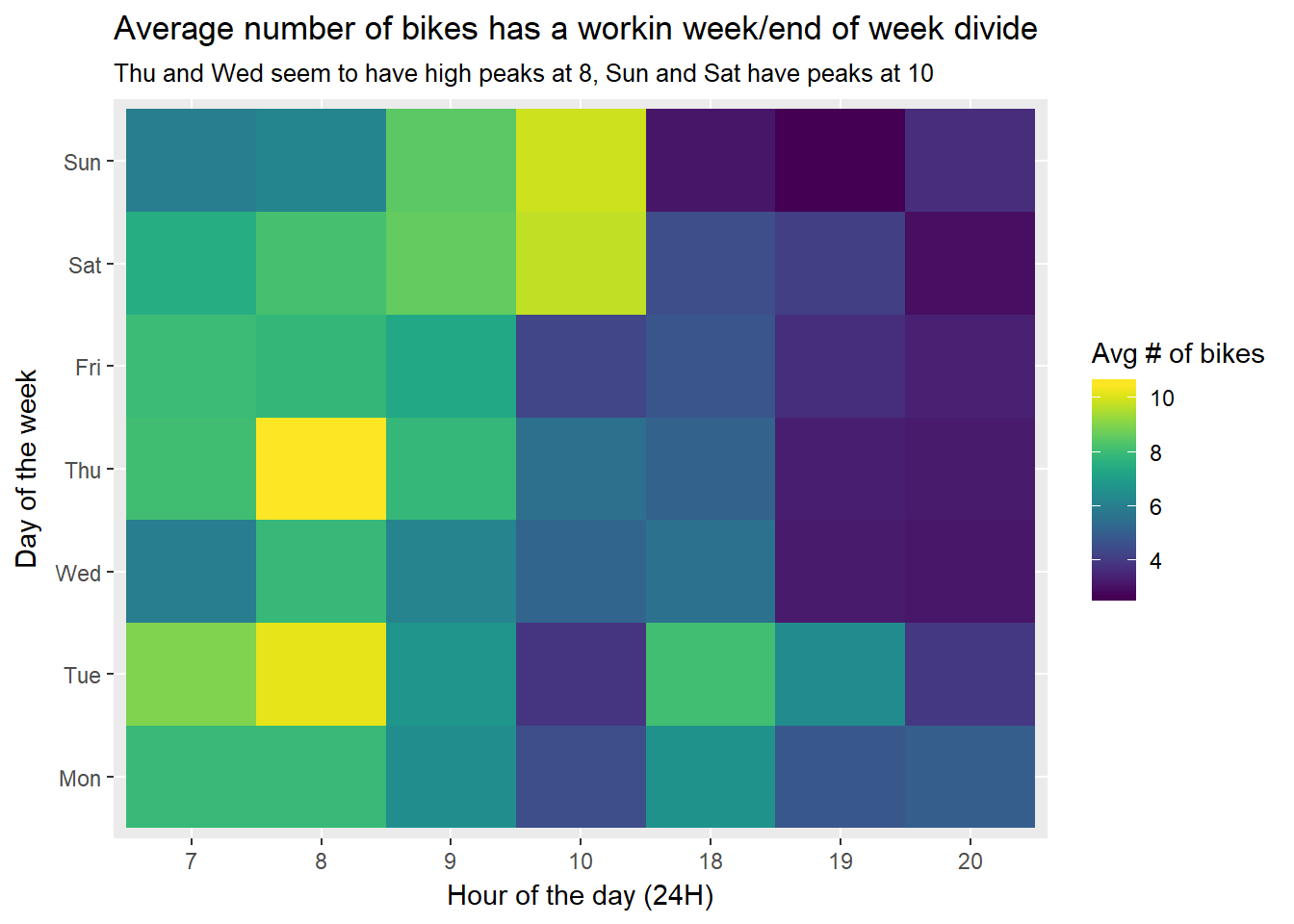
p2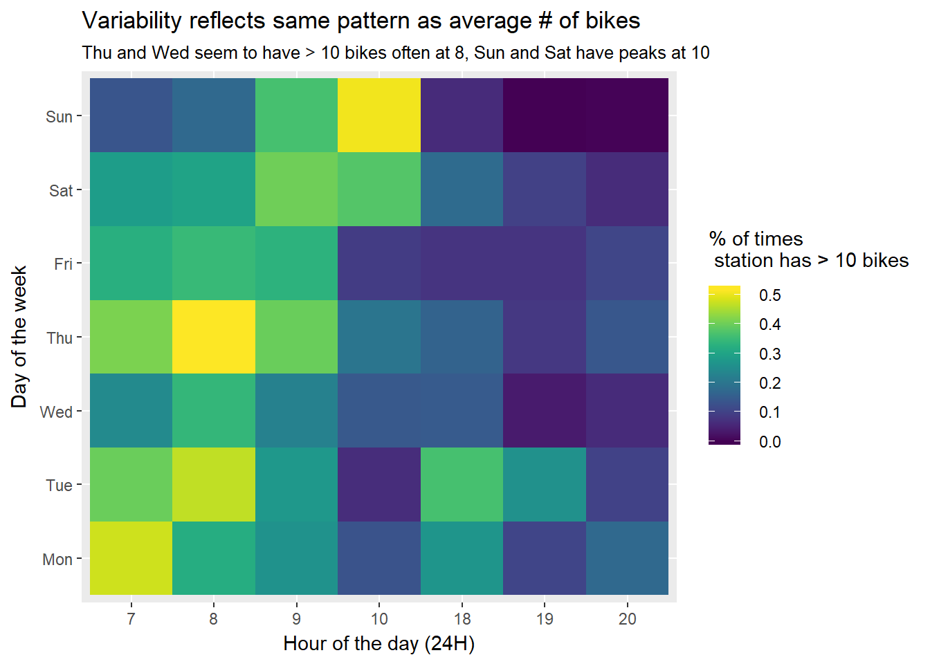
Similarly, we can see whether there’s a clear morning/evening divide by looking at the percentage of bikes for every day in the evening and the morning.
bicing %>%
  mutate(hour = lubridate::hour(time),
         day = lubridate::wday(time, label = TRUE, week_start = TRUE),
         morning_evening = ifelse(hour <= 10, "Morning", "Evening")) %>%
  ggplot(aes(day, bikes, fill = morning_evening)) +
  geom_col(position = "fill") +
  labs(x = "Day of the week",
       y = "% of bikes",
       title = '# of bikes increases linearly through out the week',
       fill = 'Time of day')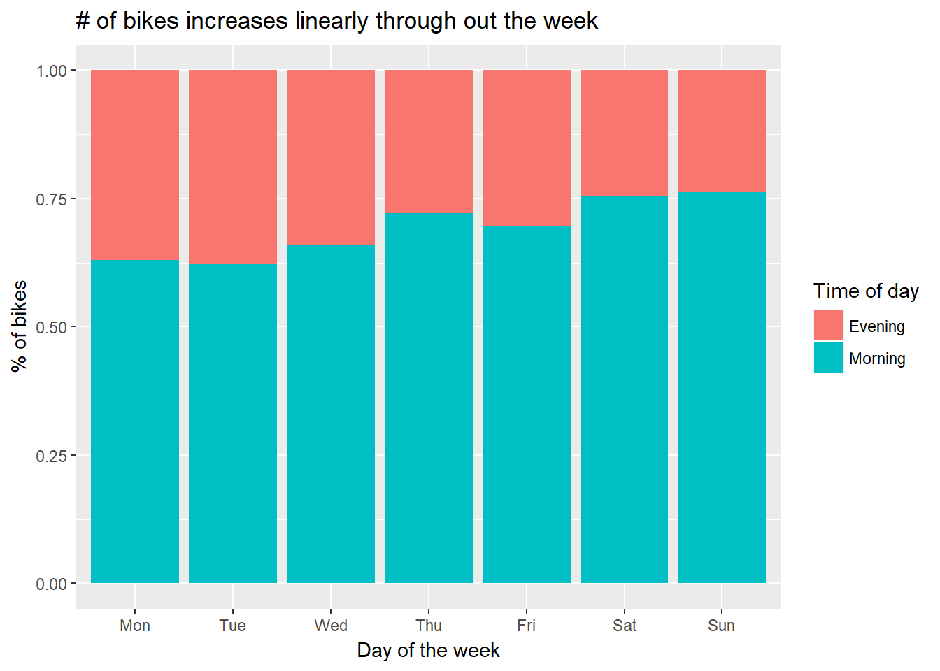
Alright, so we got that down. So far:
There’s more taking and droping happening in the first few days of the week than in the rest
Weekdays and weekends have different patterns in bike usage; namely that bike usage is higher in earlier in the week than in the weekends.
More bikes are taken in the early days of the weeks than in the latter parts.
Following the previous conclusion, I had the itching of figuring out the rate at which bicycles are taken out by hour. This we can depart from the total or average number of bikes, to actual rate of picking/droping bikes. This can help to pinpoint specific times at which we should avoid going or droping a bike.
What’s the rate at which bicycles are being taken out by hour? At which time is the station emptying out quicker?
I’ve computed a metric that calculates the percentage of minutes that there’s changes in the station.
intm_df <-
  bicing %>%
  mutate(hour = as.factor(lubridate::hour(time)),
         day = lubridate::wday(time, label = TRUE, week_start = TRUE)) %>%
  group_by(hour, day) %>%
  mutate(future_bike = lag(bikes)) %>%
  summarize(avg_movement = mean(bikes != future_bike, na.rm = TRUE) * 60) %>%
  ungroup()

intm_df %>%
  ggplot(aes(hour, avg_movement, colour = day, group = day)) +
  geom_line(size = 1.2) +
  facet_wrap(~ day, ncol = 4) +
  theme_bw() +
  labs(x = 'Hour of the day (24H)',
       y = "Minutes per hour with a bicycle change",
       title = 'Weekdays have much greater bicycle usage than weekends',
       subtitle = "Wed has the busiest hour of the week at 8AM; There's activity 25 minutes out of the 60 minutes.") +
  theme(legend.position = 'none')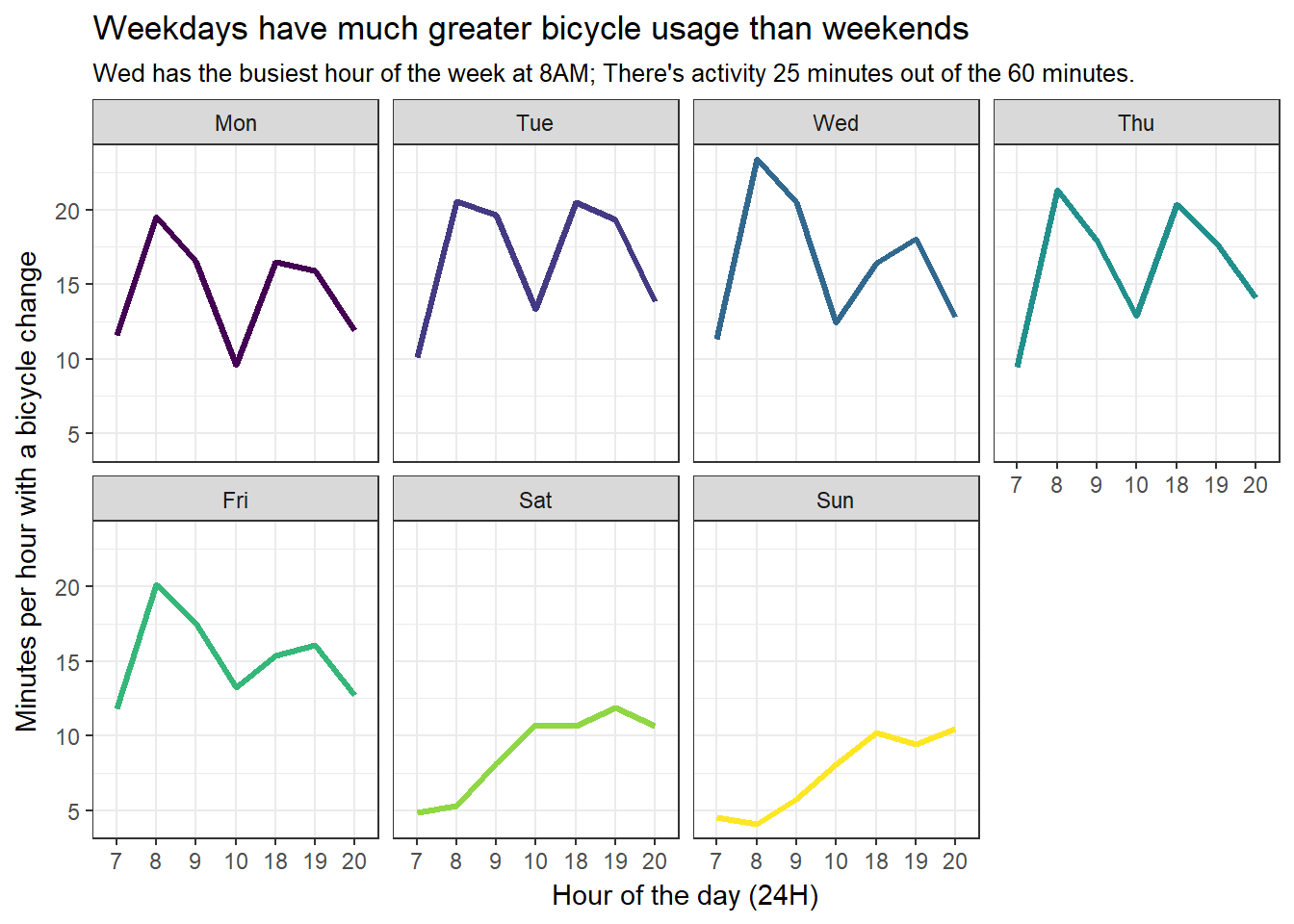
This is very interesting! This plot reverses some of the findings from before. First off, we see that there’s high variability between hours: there’s no point in looking at averages within an hour because a lot happens between minutes. For example, at 7AM and 10 AM during working days there’s very little activity regardless of the day. On the contrary, 8AM and 9AM have high bycicle usage through the working days.
This makes sense, it’s the time that people usually go to work. Also as expected, bicycle usage is low on weekend mornings and increases linearly through out the day. All in all, 8/9 AM on working days seems to be the time to avoid bicycles if you can! Eventually, in another post, I plan to investigate whether there’s minute-to-minute patterns for 8/9 AM on working days. For example, is there more activity closer to certain minutes? Like half past the hour or at exactly the hour.
Also, it seems that evenings are busy even on working days, specially on Thursdays but have very little bicycle usage on Fridays! Perhaps Catalans are ready to party and travel on the metro. On my follow up post, I also plan to see whether these patterns hold by season. I would expect summer and winter to have strong seasonal patterns.
To begin the conclusion, when are the moments when the station is empty? This will trigger me to avoid picking bicycles on those specific times.
bicing %>%
  filter(bikes == 0) %>%
  mutate(time_day = as.numeric(lubridate::hm(str_extract(time, "[0-9]{2}:[0-9]{2}")))) %>%
  ggplot(aes(x = time_day)) +
  geom_histogram()
## `stat_bin()` using `bins = 30`. Pick better value with `binwidth`.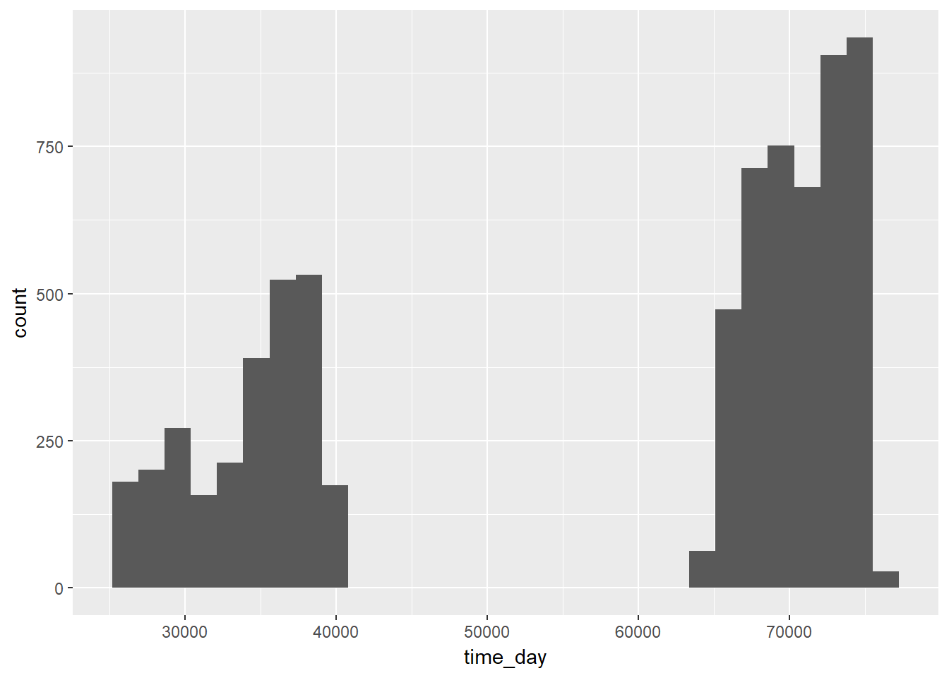
Bicing people probably prepare very well because it’s mostly empty in the evenings
The next step in the analysis is to start making predictions in waiting time. That will be the topic of my next post, in which I start to develop a modelling approach to predict the time you’ll have to have wait until a bicycle arrives or leaves. As a very simple exercise, I wanted to predict check whether I can predict when the station will be empty? I tried a simple logistic regression just to check.
empty_bicycle <-
  mutate(bicing,
         empty = ifelse(bikes == 0, 1, 0),
         hour = as.character(lubridate::hour(time)),
         day = lubridate::wday(time),
         day = as.character(day)) %>%
  select(-(1:4))

training_rows <- createDataPartition(empty_bicycle$empty, 1, p = 0.8)[[1]]

training <- empty_bicycle[training_rows, ]
test <- empty_bicycle[-training_rows, ]

mod1 <- glm(empty ~ . + day:hour, data = training, family = "binomial")

pred1 <- predict(mod1, newdata = test, type = 'response')

pred_empty <- rbinom(length(pred1), 1, prob = pred1)

confusionMatrix(test$empty, pred_empty, positive = "1")
## Confusion Matrix and Statistics
##
## Reference
## Prediction 0 1
## 0 6693 1162
## 1 1103 321
##
## Accuracy : 0.7559
## 95% CI : (0.747, 0.7646)
## No Information Rate : 0.8402
## P-Value [Acc > NIR] : 1.000
##
## Kappa : 0.0762
## Mcnemar's Test P-Value : 0.223
##
## Sensitivity : 0.21645
## Specificity : 0.85852
## Pos Pred Value : 0.22542
## Neg Pred Value : 0.85207
## Prevalence : 0.15982
## Detection Rate : 0.03459
## Detection Prevalence : 0.15346
## Balanced Accuracy : 0.53749
##
## 'Positive' Class : 1
## This model is terrible at predicting the emptyness of the stations as it can only predict 20% of the time. A few strategies I could check out to improve accuracy:
- Feature engineer when the bicing team picks up bicycles (because they leave them empty)
- Add more information on weather and public holidays from public API’s
- Because the cell that contains empty stations has very few cases, it might be useful to resample that sample until it reaches a similar sample size as the other cells. This might give greater certainty and I assume that there’s not a lot of variability in the pattern of empty stations, so it should be representative.
Finally, other classification models are certainly warranted. One good alternative would be a random forest, as it takes into consideration specific thresholds in the time of day when prunning the trees.
However, we also need to be aware that a model is as good as the data that’s being fit. Perhaps, we just need better data!