Scraping and visualizing How I Met Your Mother
How I Met Your Mother (HIMYM from here after) is a television series very similar to the classical ‘Friends’ series from the 90’s. Following the release of the tidy text book I was looking for a project in which I could apply these skills. I decided I would scrape all the transcripts from HIMYM and analyze patterns between characters. This post really took me to the limit in terms of web scraping and pattern matching, which was specifically what I wanted to improve in the first place. Let’s begin!
My first task was whether there was any consistency in the URL’s that stored the transcripts. If you ever watched HIMYM, we know there’s around nine seasons, each one with about 22 episodes. This makes about 200 episodes give or take. It would be a big pain to manually write down 200 complicated URL’s. Luckily, there is a way of finding the 200 links without writing them down manually.
First, we create the links for the 9 websites that contain all episodes (1 through season 9)
library(rvest)
library(tidyverse)
library(stringr)
library(tidytext)

main_url <- "http://transcripts.foreverdreaming.org"
all_pages <- paste0("http://transcripts.foreverdreaming.org/viewforum.php?f=177&start=", seq(0, 200, 25))
characters <- c("ted", "lily", "marshall", "barney", "robin")
Each of the URL’s of all_pages contains all episodes for that season (so around 22 URL’s). I also picked the characters we’re gonna concentrate for now. From here the job is very easy. We create a function that reads each link and parses the section containing all links for that season. We can do that using SelectorGadget to find the section we’re interested in. We then search for the href attribute to grab all links in that attribute and finally create a tibble with each episode together with it’s link.
episode_getter <- function(link) {
  title_reference <-
    link %>%
    read_html() %>%
    html_nodes(".topictitle") # Get the html node name with 'selector gadget'

  episode_links <-
    title_reference %>%
    html_attr("href") %>%
    gsub("^.", "", .) %>%
    paste0(main_url, .) %>%
    setNames(title_reference %>% html_text()) %>%
    enframe(name = "episode_name", value = "link")

  episode_links
}

all_episodes <- map_df(all_pages, episode_getter) # loop over all seasons and get all episode links
all_episodes$id <- 1:nrow(all_episodes)
There we go! Now we have a very organized tibble.
all_episodes
# # A tibble: 208 x 3
#    episode_name                   link                                  id
#    <chr>                          <chr>                              <int>
#  1 01x01 - Pilot                  http://transcripts.foreverdreamin~     1
#  2 01x02 - Purple Giraffe         http://transcripts.foreverdreamin~     2
#  3 01x03 - Sweet Taste of Liberty http://transcripts.foreverdreamin~     3
#  4 01x04 - Return of the Shirt    http://transcripts.foreverdreamin~     4
#  5 01x05 - Okay Awesome           http://transcripts.foreverdreamin~     5
#  6 01x06 - Slutty Pumpkin         http://transcripts.foreverdreamin~     6
#  7 01x07 - Matchmaker             http://transcripts.foreverdreamin~     7
#  8 01x08 - The Duel               http://transcripts.foreverdreamin~     8
#  9 01x09 - Belly Full of Turkey   http://transcripts.foreverdreamin~     9
# 10 01x10 - The Pineapple Incident http://transcripts.foreverdreamin~    10
# # ... with 198 more rows
The remaining part is to actually scrape the text from each episode. We can work that out for a single episode and then turn that into a function and apply for all episodes.
episode_fun <- function(file) {

  file %>%
    read_html() %>%
    html_nodes(".postbody") %>%
    html_text() %>%
    str_split("\n|\t") %>%
    .[[1]] %>%
    data_frame(text = .) %>%
    filter(str_detect(text, ""), # Lots of empty spaces
           !str_detect(text, "^\\t"), # Lots of lines with \t to delete
           !str_detect(text, "^\\[.*\\]$"), # Text that start with brackets
           !str_detect(text, "^\\(.*\\)$"), # Text that starts with parenthesis
           str_detect(text, "^*.:"), # I want only lines with start with dialogue (:)
           !str_detect(text, "^ad")) # Remove lines that start with ad (for 'ads', the link of google ads)
}
The above function reads each episode, turns the html text into a data frame and organizes it clearly for text analysis. For example:
episode_fun(all_episodes$link[15])
# # A tibble: 195 x 1
#    text
#    <chr>
#  1 Ted from 2030: Kids, something you might not know about your Uncle Mar~
#  2 "Ted: You don't have to shout out \"poker\" when you win."
#  3 Marshall: I know. It's just fun to say.
#  4 "Ted from 2030: We all finally agreed Marshall should be running our g~
#  5 "Marshall: It's called \"Marsh-gammon.\" It combines all the best feat~
#  6 Robin: Backgammon, obviously.
#  7 "Marshall: No. Backgammon sucks. I took the only good part of backgamm~
#  8 Lily: I'm so excited Victoria's coming.
#  9 Robin: I'm going to go get another round.
# 10 Ted: Okay, I want to lay down some ground rules for tonight. Barney, I~
# # ... with 185 more rows
We now have a data frame with only dialogue for each character. We need to apply that function to each episode and bind everything together. We first apply the function to every episode.
all_episodes$text <- map(all_episodes$link, episode_fun)The text list-column is an organized list with text for each episode. However, manual inspection of some episodes actually denotes a small error that limits our analysis greatly. Among the main interests of this document is to study relationships and presence between characters. For that, we need each line of text to be accompanied by the character who said it. Unfortunately, some of these scripts don’t have that.
For example, check any episode from season 8 and 9. The writer didn’t write the dialogue and just rewrote the lines. There’s nothing we can do so far to improve that and we’ll be excluding these episodes. This pattern is also present in random episodes like in season 4 or season 6. We can exclude chapters based on the number of lines we parsed. On average, each of these episodes has about 200 lines of dialogue. Anything significantly lower, like 30 or 50 lines, is an episode which doesn’t have a lot of dialogue.
all_episodes$count <- map_dbl(all_episodes$text, nrow)We can extend the previous tibble to be a bit more organized by separating the episode-season column into separate season and episo numbers.
all_episodes <-
  all_episodes %>%
  separate(episode_name, c("season", "episode"), "-", extra = "merge") %>%
  separate(season, c("season", "episode_number"), sep = "x")
Great! We now have a very organized tibble with all the information we need. Next step is to actually break down the lines into words and start looking for general patterns. We can do that by looping through all episodes that have over 100 lines (just an arbitrary threshold) and unnesting each line for each valid character.
lines_characters <-
  map(filter(all_episodes, count > 100) %>% pull(text), ~ {
    # only loop over episodes that have over 100 lines
    .x %>%
      separate(text, c("character", "text"), sep = ":", extra = 'merge') %>%
      # separate character dialogue from actual dialogo
      unnest_tokens(character, character) %>%
      filter(str_detect(character, paste0(paste0("^", characters, "$"), collapse = "|"))) %>%
      # only count the lines of our chosen characters
      mutate(episode_lines_id = 1:nrow(.))
  }) %>%
  setNames(filter(all_episodes, count > 100) %>% # name according to episode
             unite(season_episode, season, episode_number, sep = "x") %>%
             pull(season_episode)) %>%
  enframe() %>%
  unnest() %>%
  mutate(all_lines_id = 1:nrow(.))
Ok, our text is sort of ready. Let’s remove some bad words.
words_per_character <-
  lines_characters %>%
  unnest_tokens(word, text) %>% # expand all sentences into words
  anti_join(stop_words) %>% # remove bad words
  filter(!word %in% characters) %>% # only select characters we're interested
  arrange(name) %>%
  separate(name, c("season", "episode"), sep = "x", remove = FALSE) %>%
  mutate(name = factor(name, ordered = TRUE),
         season = factor(season, ordered = TRUE),
         episode = factor(episode, ordered = TRUE)) %>%
  filter(season != "07")
Just to make sure, let’s look at the tibble.
words_per_character
# # A tibble: 88,174 x 7
#    name     season episode character episode_lines_id all_lines_id word
#    <ord>    <ord>  <ord>   <chr>                <int>        <int> <chr>
#  1 "01x01 " 01     "01 "   marshall                 1            1 ring
#  2 "01x01 " 01     "01 "   marshall                 1            1 marry
#  3 "01x01 " 01     "01 "   ted                      2            2 perfect
#  4 "01x01 " 01     "01 "   ted                      2            2 engaged
#  5 "01x01 " 01     "01 "   ted                      2            2 pop
#  6 "01x01 " 01     "01 "   ted                      2            2 champa~
#  7 "01x01 " 01     "01 "   ted                      2            2 drink
#  8 "01x01 " 01     "01 "   ted                      2            2 toast
#  9 "01x01 " 01     "01 "   ted                      2            2 kitchen
# 10 "01x01 " 01     "01 "   ted                      2            2 floor
# # ... with 88,164 more rows
Perfect! One row per word, per character, per episode with the id of the line of the word.
Alright, let’s get our hands dirty. First, let visualize the presence of each character in terms of words over time.
# Filtering position of first episode of all seasons to
# position the X axis in the next plot.
first_episodes <-
  all_episodes %>%
  filter(count > 100, episode_number == "01 ") %>%
  pull(id)

words_per_character %>%
  split(.$name) %>%
  setNames(1:length(.)) %>%
  enframe(name = "episode_id") %>%
  unnest() %>%
  count(episode_id, character) %>%
  group_by(episode_id) %>%
  mutate(total_n = sum(n),
         perc = round(n / total_n, 2)) %>%
  ggplot(aes(as.numeric(episode_id), perc, group = character, colour = character)) +
  geom_line() +
  geom_smooth(method = "lm") +
  scale_colour_discrete(guide = FALSE) +
  scale_x_continuous(name = "Seasons",
                     breaks = first_episodes, labels = paste0("S", 1:7)) +
  scale_y_continuous(name = "Percentage of words per episode") +
  theme_minimal() +
  facet_wrap(~ character, ncol = 3)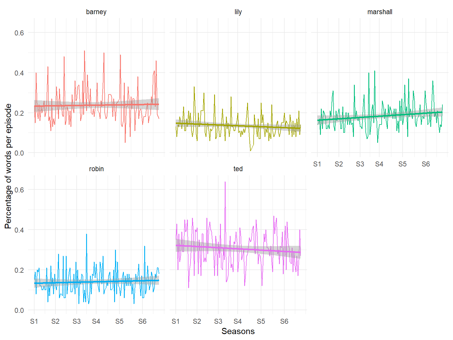
Ted is clearly the character with the highest number of words per episode followed by Barney. Lily and Robin, the only two women have very low presence compared to the men. In fact, if one looks closely, Lily seemed to have decreased slightly over time, having an all time low in season 4. Marshall, Lily’s partner in the show, does have much lower presence than both Barney and Ted but he has been catching up over time.
We also see an interesting pattern where Barney has a lot of peaks, suggesting that in some specific episodes he gains predominance, where Ted has an overall higher level of words per episode. And when Ted has peaks, it’s usually below its trend-line.
Looking at the distribution:
# devtools::install_github("clauswilke/ggjoy")
library(ggjoy)

words_per_character %>%
  split(.$name) %>%
  setNames(1:length(.)) %>%
  enframe(name = "episode_id") %>%
  unnest() %>%
  count(season, episode_id, character) %>%
  group_by(episode_id) %>%
  mutate(total_n = sum(n),
         perc = round(n / total_n, 2)) %>%
  ggplot(aes(x = perc, y = character, fill = character)) +
  geom_joy(scale = 0.85) +
  scale_fill_discrete(guide = F) +
  scale_y_discrete(name = NULL, expand=c(0.01, 0)) +
  scale_x_continuous(name = "Percentage of words", expand=c(0.01, 0)) +
  ggtitle("Percentage of words per season") +
  facet_wrap(~ season, ncol = 7) +
  theme_minimal()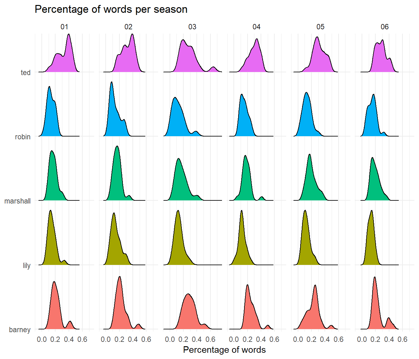
we see the differences much clearer. For example, we see Barney’s peaks through out every season with Season 6 seeing a clear peak of 40%. On the other hand, we see that their distributions don’t change that much over time! Suggesting that the presence of each character is very similar in all seasons. Don’t get me wrong, there are differences like Lily in Season 2 and then in Season 6, but in overall terms the previous plot suggests no increase over seasons, and this plot suggests that between seasons, there’s not a lot of change in their distributions that affects the overall mean.
If you’ve watched the TV series, you’ll remember Barney always repeating one similar trademark word: legendary! Although it is a bit cumbersome for us to count the number of occurrences of that sentence once we unnested each sentence, we can at least count the number of words per character and see whether some characters have particular words.
count_words <-
  words_per_character %>%
  filter(!word %in% characters) %>%
  count(character, word, sort = TRUE)

count_words %>%
  group_by(character) %>%
  top_n(20) %>%
  ggplot(aes(reorder(word, n), n)) +
  geom_col(alpha = 0.8) +
  coord_flip() +
  facet_wrap(~ character, scales = "free_y")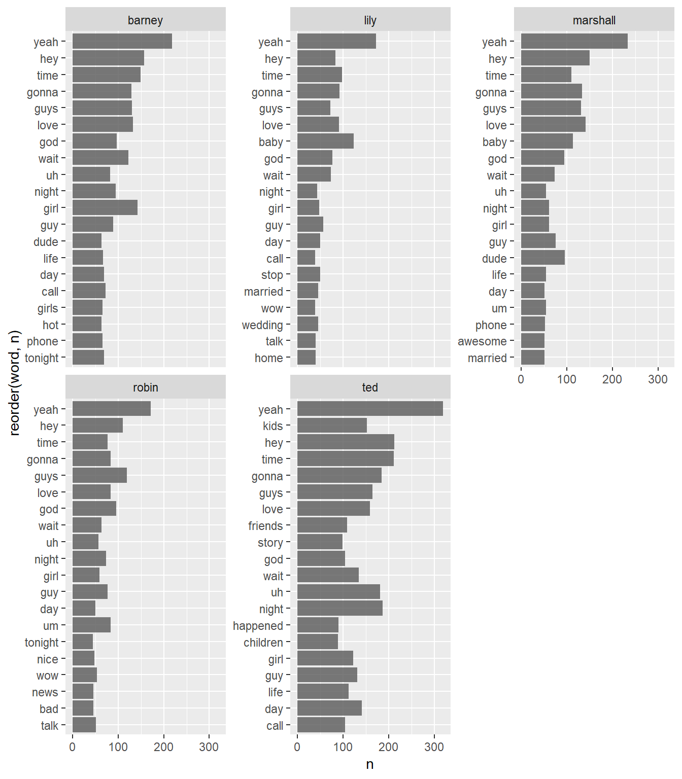
Here we see that a lot of the words we capture are actually nouns or expressions which are common to everyone, such as ‘yeah’, ‘hey’ or ‘time’. We can weight down commonly used words for other words which are important but don’t get repeated a lot. We can exclude those words using bind_tf_idf(), which for each character decreases the weight for commonly used words and increases the weight for words that are not used very much in a collection or corpus of documents (see 3.3 in http://tidytextmining.com/tfidf.html).
count_words %>%
  bind_tf_idf(word, character, n) %>%
  arrange(desc(tf_idf)) %>%
  group_by(character) %>%
  top_n(20) %>%
  ggplot(aes(reorder(word, n), n)) +
  geom_col(alpha = 0.8) +
  coord_flip() +
  facet_wrap(~ character, scales = "free_y")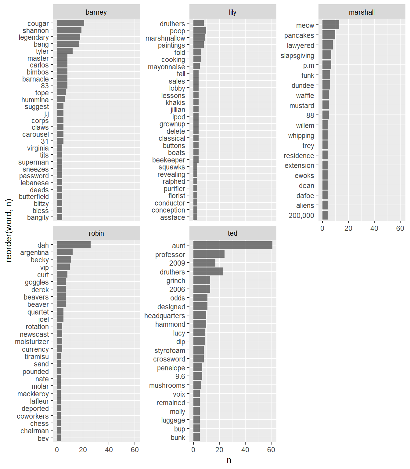
Now Barney has a very distinctive word usage, one particularly sexist with words such as couger, bang and tits. Also, we see the word legendary as the thirdly repeated word, something we were expecting! On the other hand, we see Ted with things like professor (him), aunt (because of aunt Lily and such).
Knowing that Ted is the main character in the series is no surprise. To finish off, we’re interested in knowing which characters are related to each other. First, let’s turn the data frame into a suitable format.
Here we turn all lines to lower case and check which characters are present in the text of each dialogue. The loop will return a vector of logicals whether there was a mention of any of the characters. For simplicity I exclude all lines where there is more than 1 mention of a character, that is, 2 or more characters.
lines_characters <-
  lines_characters %>%
  mutate(text = str_to_lower(text))

rows_fil <-
  map(characters, ~ str_detect(lines_characters$text, .x)) %>%
  reduce(`+`) %>%
  ifelse(. >= 2, 0, .) # excluding sentences which have 2 or more mentions for now
  # ideally we would want to choose to count the number of mentions
  # per line or randomly choose another a person that was mentioned.
Now that we have the rows that have a mention of another character, we subset only those rows. Then we want know which character was mentioned in which line. I loop through each line and test which character is present in that specific dialogue line. The loop returns the actual character name for each dialogue. Because we already filtered lines that have a character name mentioned, the loop should return a vector of the same length.
character_relation <-
  lines_characters %>%
  filter(as.logical(rows_fil)) %>%
  mutate(who_said_what =
           map_chr(.$text, ~ { # loop over all each line
             who_said_what <- map_lgl(characters, function(.y) str_detect(.x, .y))
             # loop over each character and check whether he/she was mentioned
             # in that line
             characters[who_said_what]
             # subset the character that matched
           }))
Finally, we plot the relationship using the ggraph package.
library(ggraph)
library(igraph)

character_relation %>%
  count(character, who_said_what) %>%
  graph_from_data_frame() %>%
  ggraph(layout = "linear", circular = TRUE) +
  geom_edge_arc(aes(edge_alpha = n, edge_width = n),
                width = 2.5, show.legend = FALSE) +
  geom_node_text(aes(label = name), repel = TRUE) +
  theme_void()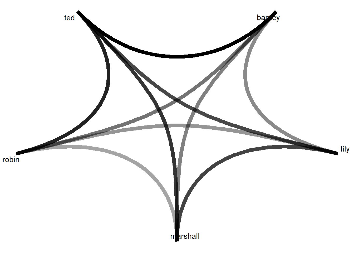
A very clear pattern emerges. There is a strong relationship between Robin and Barney towards Ted. In fact, their direct relationship is very weak, but both are very well connected to Ted. On the other hand, Marshall and Lily are also reasonably connected to Ted but with a weaker link. Both of them are indeed very connected, as should be expected since they were a couple in the TV series.
We also see that the weakest members of the group are Robin and Barney with only strong bonds toward Ted but no strong relationship with the other from the group. Overall, there seems to be a division: Marshall and Lily hold a somewhat close relationship with each other and towards Ted and Barney and Robin tend to be related to Ted but no one else.
As a follow-up question, is this pattern of relationships the same across all seasons? We can do that very quickly by filtering each season using the previous plot.
library(cowplot)

# Loop through each season
seasons <- paste0(0, 1:7)

all_season_plots <- lapply(seasons, function(season_num) {

  set.seed(2131)

  character_relation %>%
    # Extract the season number from the `name` column
    mutate(season = str_replace_all(character_relation$name, "x(.*)$", "")) %>%
    filter(season == season_num) %>%
    count(character, who_said_what) %>%
    graph_from_data_frame() %>%
    ggraph(layout = "linear", circular = TRUE) +
    geom_edge_arc(aes(edge_alpha = n, edge_width = n),
                  width = 2.5, show.legend = FALSE) +
    geom_node_text(aes(label = name), repel = TRUE) +
    theme_void()
})

# Plot all graphs side-by-side
cowplot::plot_grid(plotlist = all_season_plots, labels = seasons)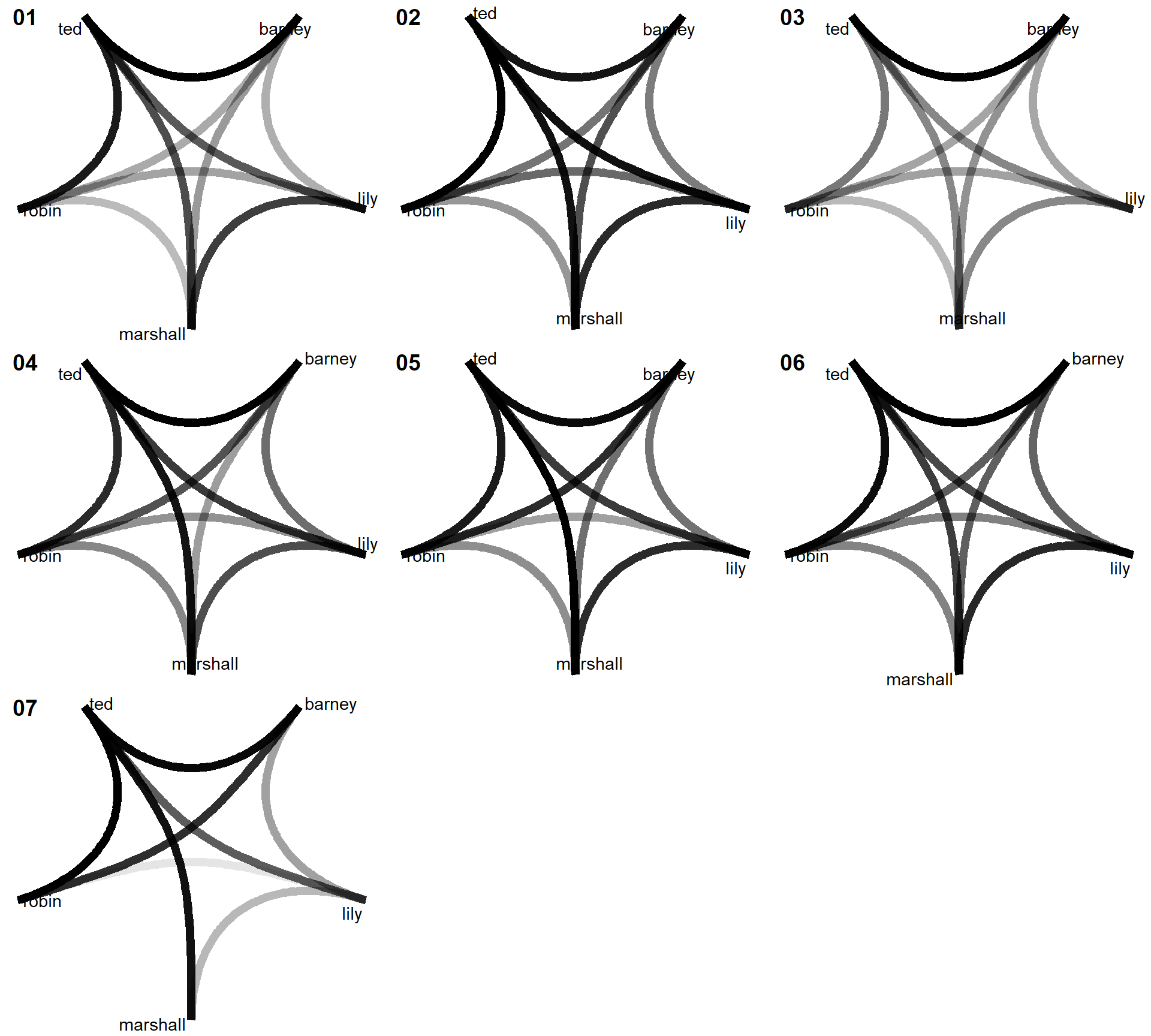
There are reasonable changes for all non-Ted relationship! For example, for season 2 the relationship Marshall-Lily-Ted becomes much stronger and it disappears in season 3. Let’s remember that these results might be affected by the fact that I excluded some episodes because of low number of dialogue lines. Keeping that in mind, we also see that for season 7 the Robin-Barney relationship became much stronger (is this the season the started dating?). All in all, the relationships don’t look dramatically different from the previous plot. Everyone seems to be strongly related to Ted. The main difference is the changes in relationship between the other members of the cast.
This dataset has a lot of potential and I’m sure I’ve scratched the surface of what one can do with this data. I encourage anyone interested in the topic to use the code to analyze the data further. One idea I might explore in the future is to build a model that attempts to predict who said what for all dialogue lines that didn’t have a character member. This can be done by extracting features from all sentences and using these patterns try to classify which. Any feedback is welcome, so feel free to message me at cimentadaj@gmail.com