perccalc package
Reardon (2011) introduced a very interesting concept in which he calculates percentile differences from ordered categorical variables. He explains his procedure very much in detail in the appendix of the book chapter but no formal implementation has been yet available on the web. With this package I introduce a function that applies the procedure, following a step-by-step Stata script that Sean Reardon kindly sent me.
In this vignette I show you how to use the function and match the results to the Stata code provided by Reardon himself.
For this example, we’ll use a real world data set, one I’m very much familiar with: PISA. We’ll use the PISA 2012 wave for Germany because it asked parents about their income category. For this example we’ll need the packages below.
# install.packages(c("devtools", "matrixStats", "tidyverse"))
# devtools::install_github("pbiecek/PISA2012lite")

library(matrixStats)
library(tidyverse)
library(haven)
library(PISA2012lite)
If you haven’t installed any of the packages above, uncomment the first two lines to install them. Beware that the PISA2012lite package contains the PISA 2012 data and takes a while to download.
Let’s prepare the data. Below we filter only German students, select only the math test results and calculate the median of all math plausible values to get one single math score. Finally, we match each student with their corresponding income data from their parents data and their sample weights.
ger_student <- student2012 %>%
  filter(CNT == "Germany") %>%
  select(CNT, STIDSTD, matches("^PV*.MATH$")) %>%
  transmute(CNT, STIDSTD,
            avg_score = rowMeans(student2012[student2012$CNT == "Germany", paste0("PV", 1:5, "MATH")]))

ger_parent <-
  parent2012 %>%
  filter(CNT == "Germany") %>%
  select(CNT, STIDSTD, PA07Q01)

ger_weights <-
  student2012weights %>%
  filter(CNT == "Germany") %>%
  select(CNT, STIDSTD, W_FSTUWT)

dataset_ready <-
  ger_student %>%
  left_join(ger_parent, by = c("CNT", "STIDSTD")) %>%
  left_join(ger_weights, by = c("CNT", "STIDSTD")) %>%
  as_tibble() %>%
  rename(income = PA07Q01,
         score = avg_score,
         wt = W_FSTUWT) %>%
  select(-CNT, -STIDSTD)
The final results is this dataset:
## # A tibble: 10 x 3
##   score income            wt
##   <dbl> <fct>          <dbl>
## 1  440. Less than <$A>  137.
## 2  523. Less than <$A>  170.
## 3  291. Less than <$A>  162.
## 4  437. Less than <$A>  162.
## 5  367. Less than <$A>  115.
## # ... with 5 more rows
This is the minimum dataset that the function will accept. This means that it needs to have at least a categorical variable and a continuous variable (the vector of weights is optional).
The package is called perccalc, short for percentile calculator and we can install and load it with this code:
install.packages("perccalc", repo = "https://cran.rediris.es/")
## package 'perccalc' successfully unpacked and MD5 sums checked
##
## The downloaded binary packages are in
##  C:\Users\cimentadaj\AppData\Local\Temp\RtmpYFnDzN\downloaded_packages
library(perccalc)
The package has two functions, which I’ll show some examples. The first one is called perc_diff and it’s very easy to use, we just specify the data, the name of the categorical and continuous variable and the percentile difference we want.
Let’s put it to use!
perc_diff(dataset_ready, income, score, percentiles = c(90, 10))
## Error: is_ordered_fct is not TRUE
I generated that error on purpose to raise a very important requirement of the function. The categorical variable needs to be an ordered factor (categorical). It is very important because otherwise we could be calculating percentile differences of categorical variables such as married, single and widowed, which doesn’t make a lot of sense.
We can turn it into an ordered factor with the code below.
dataset_ready <-
  dataset_ready %>%
  mutate(income = factor(income, ordered = TRUE))
Now it’ll work.
perc_diff(dataset_ready, income, score, percentiles = c(90, 10))
## difference         se
##   97.00706    8.74790
We can play around with other percentiles
perc_diff(dataset_ready, income, score, percentiles = c(50, 10))
## difference         se
##  58.776200   8.291083
And we can add a vector of weights
perc_diff(dataset_ready, income, score, weights = wt, percentiles = c(90, 10))
## difference         se
##  95.228517   8.454902
Now, how are we sure that these estimates are as accurate as the Reardon (2011) implementation? We can compare the Stata ouput using this data set.
# Saving the dataset to a path
dataset_ready %>%
  write_dta(path = "/Users/cimentadaj/Downloads/pisa_income.dta", version = 13)
Running the code below using the pisa_income.dta..
*--------
use "/Users/cimentadaj/Downloads/pisa_income.dta", clear

tab income, gen(inc)
*--------

/*-----------------------
    Making a data set that has
    one observation per income category
    and has mean and se(mean) in each category
    and percent of population in the category
------------------------*/

tempname memhold
tempfile results
postfile `memhold' income mean se_mean per using `results'

forv i = 1/6 {
    qui sum inc`i' [aw=wt]
    loc per`i' = r(mean)

    qui sum score if inc`i'==1

    if `r(N)'>0 {
        qui regress score if inc`i'==1 [aw=wt]
        post `memhold' (`i') (_b[_cons]) (_se[_cons]) (`per`i'')

    }
}
postclose `memhold'

/*-----------------------
    Making income categories
    into percentiles
------------------------*/


    use `results', clear

    sort income
    gen cathi = sum(per)
    gen catlo = cathi[_n-1]
    replace catlo = 0 if income==1
    gen catmid = (catlo+cathi)/2

    /*-----------------------
        Calculate income
        achievement gaps
    ------------------------*/

    sort income

    g x1 = catmid
    g x2 = catmid^2 + ((cathi-catlo)^2)/12
    g x3 = catmid^3 + ((cathi-catlo)^2)/4

    g cimnhi = mean + 1.96*se_mean
    g cimnlo = mean - 1.96*se_mean

    reg mean x1 x2 x3 [aw=1/se_mean^2]

    twoway (rcap cimnhi cimnlo catmid) (scatter mean catmid) ///
        (function y = _b[_cons] + _b[x1]*x + _b[x2]*x^2 + _b[x3]*x^3, ran(0 1))

    loc hi_p = 90
    loc lo_p = 10

    loc d1 = [`hi_p' - `lo_p']/100
    loc d2 = [(`hi_p')^2 - (`lo_p')^2]/(100^2)
    loc d3 = [(`hi_p')^3 - (`lo_p')^3]/(100^3)

    lincom `d1'*x1 + `d2'*x2 + `d3'*x3
    loc diff`hi_p'`lo_p' = r(estimate)
    loc se`hi_p'`lo_p' = r(se)

    di "`hi_p'-`lo_p' gap:     `diff`hi_p'`lo_p''"
    di "se(`hi_p'-`lo_p' gap): `se`hi_p'`lo_p''"
I get that the 90/10 difference is 95.22 with a standard error of 8.45. Does it sound familiar?
perc_diff(dataset_ready, income, score, weights = wt, percentiles = c(90, 10))
## difference         se
##  95.228517   8.454902
The second function of the package is called perc_dist and instead of calculating the difference of two percentiles, it returns the score and standard error of every percentile. The arguments of the function are exactly the same but without the percentiles argument, because this will return the whole set of percentiles.
perc_dist(dataset_ready, income, score)
## # A tibble: 100 x 3
##   percentile estimate std.error
##        <int>    <dbl>     <dbl>
## 1          1     3.69      1.33
## 2          2     7.28      2.59
## 3          3    10.8       3.79
## 4          4    14.1       4.93
## 5          5    17.4       6.01
## # ... with 95 more rows
We can also add the optional set of weights and graph it:
perc_dist(dataset_ready, income, score, wt) %>%
  mutate(ci_low = estimate - 1.96 * std.error,
         ci_hi = estimate + 1.96 * std.error) %>%
  ggplot(aes(percentile, estimate)) +
  geom_point() +
  geom_errorbar(aes(ymin = ci_low, ymax = ci_hi))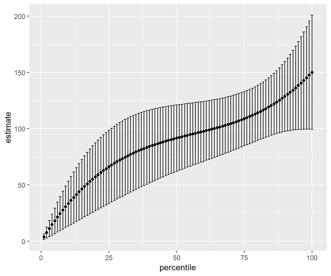
Please note that for calculating the difference between two percentiles it is more accurate to use the perc_diff function. The perc_diff calculates the difference through a linear combination of coefficients resulting in a different standard error.
For example:
perc_dist(dataset_ready, income, score, wt) %>%
  filter(percentile %in% c(90, 10)) %>%
  summarize(diff = diff(estimate),
            se_diff = diff(std.error))
## # A tibble: 1 x 2
##    diff se_diff
##   <dbl>   <dbl>
## 1  95.2    5.68
compared to
perc_diff(dataset_ready, income, score, weights = wt, percentiles = c(90, 10))
## difference         se
##  95.228517   8.454902
They both have the same point estimate but a different standard error.
I hope this was a convincing example, I know this will be useful for me. All the intelectual ideas come from Sean Reardon and the Stata code was written by Sean Reardon, Ximena Portilla, and Jenna Finch. The R implemention is my own work.
You can find the package repository here.
- Reardon, Sean F. “The widening academic achievement gap between the rich and the poor: New evidence and possible explanations.” Whither opportunity (2011): 91-116.