Simulations and model predictions in R

I was on a flight from Asturias to Barcelona yesterday and I finally had some free time to open Gelman and Hill’s book and submerge in some studying. After finishing the chapter on simulations, I tried doing the first exercise and enjoyed it very much.

The exercise goes as follows:

Discrete probability simulation: suppose that a basketball player has a 60% chance of making a shot, and he keeps taking shots until he misses two in a row. Also assume his shots are independent (so that each shot has 60% probability of success, no matter what happened before).

1. Write an R function to simulate this process.

2. Put the R function in a loop to simulate the process 1000 times. Use the simulation to estimate the mean, standard deviation, and distribution of the total number of shots that the player will take.

3. Using your simulations, make a scatterplot of the number of shots the player will take and the proportion of shots that are successes.

Below you can find my answer with some comments on how I did it:

# a)
# The probs argument sets the probability of making a shot. In this case it'll be 0.60
thrower <- function(probs) {
  vec <- replicate(2, rbinom(1, 1, probs)) 
  # create a vector with two random numbers of either 1 or 0,
  # with a probability of probs for 1
  
  # While the sum of the last and the second-last element is not 0
  while ((vec[length(vec)] + vec[length(vec) - 1]) != 0) { 
    
      vec <- c(vec, rbinom(1, 1, probs))
      # keep adding random shots with a probability of probs
  }
return(vec)
}
# The loop works because whenever the sum of the last two elements is 0,
# then the last two elements must be 0 meaning that the player missed two
# shots in a row.

# test
thrower(0.6)

##  [1] 1 0 1 0 1 1 1 1 1 1 1 1 0 1 1 1 0 1 1 1 0 1 1 0 1 1 1 0 0

# 0 1 0 1 0 0
# Last two elements are always zero

# b)
attempts <- replicate(1000, thrower(0.60))
mean(sapply(attempts, length)) 

## [1] 8.501

# mean number of shots until two shots are missed in a row

sd(sapply(attempts, length)) 

## [1] 7.158019

# standard deviation of shots made
# until two shots are missed in a row

hist(sapply(attempts, length)) # distribution of shots made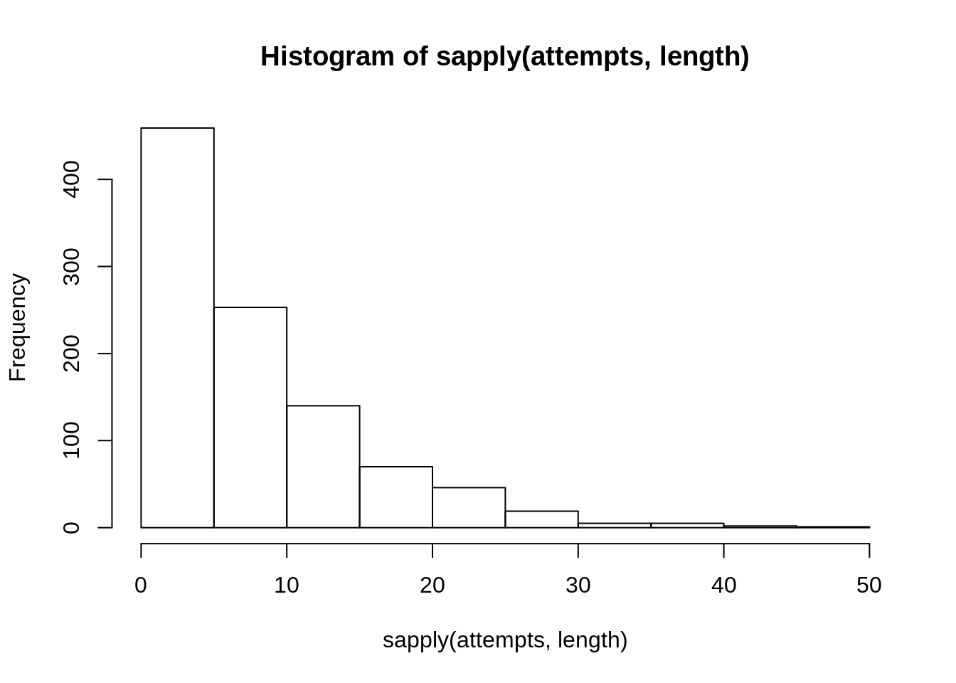

# c)
df <- cbind(sapply(attempts, mean), sapply(attempts, length)) 
# data frame with % of shots made and number of shots thrown
plot(df[, 2], df[, 1])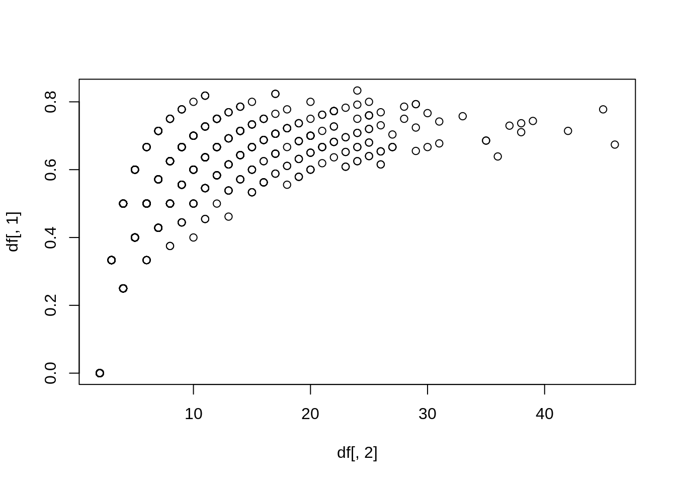

That was fun. I think the key take away here is that you can use these type of simulations to asses the accuracy of model predictions, for example. If you have the probability of being in either 1 or 0 in any dependent variable, then simulation can help determine its reliability by looking at the distribution of the replications.

Whenever I have some free time I’ll go back to the next exercises.